We are excited to announce our new RL Tuner algorithm, a method for enchancing the performance of an LSTM trained on data using Reinforcement Learning (RL). We create an RL reward function that teaches the model to follow certain rules, while still allowing it to retain information learned from data. We use RL Tuner to teach concepts of music theory to an LSTM trained to generate melodies. The two videos below show samples from the original LSTM model, and the same model enchanced using RL Tuner.
Introduction
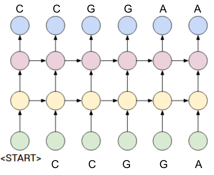
When I joined Magenta as an intern this summer, the team was hard at work on developing better ways to train Recurrent Neural Networks (RNNs) to generate sequences of notes. As you may remember from previous posts, these models typically consist of a Long Short-Term Memory (LSTM) network trained on monophonic melodies. This means that melodies are fed into the network one note at a time, and it is trained to predict the next note in the sequence. The figure on the left shows a simplified version of this type of network unrolled over time, in which it is being trained on the first 6 notes of “Twinkle Twinkle Little Star”. From now on, I’ll refer to this type of model as a Note RNN.
A Note RNN is conceptually similar to a Character RNN, a popular model for generating text, one character at a time. While both types of models can produce impressive results, they have some frustrating limitations. They both suffer from common failure modes, such as continually repeating the same token. Further, the sequences produced by the models tend to lack a consistent global structure. To see this more clearly, take a look at the text below, which was generated by a Character RNN trained on Wikipedia markdown data (taken from Graves, 2013):
The ‘'’Rebellion’’’ (‘‘Hyerodent’’) is [[literal]], related mildly older than old half sister, the music, and morrow been much more propellent. All those of [[Hamas (mass)|sausage trafficking]]s were also known as [[Trip class submarine|“Sante” at Serassim]]; “Verra” as 1865-682-831 is related to ballistic missiles. While she viewed it friend of Halla equatorial weapons of Tuscany, in [[France]], from vaccine homes to "individual", among [[slavery|slaves]](such as artistual selling of factories were renamed English habit of twelve years.)
While the model has learned how to correctly spell English words, some markdown syntax, and even mostly correct grammatical structure, sentences don’t seem to follow a consistent thought. The text wonders rapidly from topic to topic, discussing everything from sisters to submarines to Tuscany, slavery, and factories, all in one short paragraph. This type of global incoherence is typical of the melodies produced by a vanilla Note RNN as well. They do not maintain a consistent musical structure, and can sound wandering and random.
Music is an interesting test-bed for sequence generation, in that musical compositions adhere to a relatively well-defined set of structural rules. Any beginning music student learns that groups of notes belong to keys, chords follow progressions, and songs have consistent structures made up of musical phrases. So what if we could teach a Note RNN these kinds of musical rules, while still allowing it to learn patterns from music it hears in the world?
This is the idea behind the RL Tuner model I will describe in this post. We take a trained Note RNN and teach it concepts of music theory using Reinforcement Learning (RL). RL can allow a network to learn some non-differentiable reward function. In this case, we define a set of music theory rules, and produce rewards based on whether the model’s compositions adhere to those rules. However, to ensure that the model can remember the note probabilities it originally learned from data, we keep a second, fixed copy of the Note RNN which we call the Reward RNN. The Reward RNN is used to compute the probability of playing the next note as learned by the original Note RNN. We augment our music theory rewards with this probability value, so that the total reward reflects both our music theory constraints and information learned from data.
We show that this approach allows the model to maintain information about the note probabilities learned from data, while significantly improving the behaviors of the Note RNN targeted by the music theory rewards. For example, before training with RL, 63.3% of notes produced by the Note RNN belonged to some excessively repeated segment of notes; after RL, 0.0-0.03% of notes were excessively repeated. Since excessively repeating tokens is a problem in other domains as well (e.g. text generation), we believe our approach could have broader applications. But does it actually work to produce better music? We conducted a user study and found that people find the compositions produced by our three RL models significantly more musically pleasing than those of the original Note RNN. But we encourage you to judge for yourself; samples from each of the models will be provided later in this post.
The models, derivations, and results are all described in our recent research paper, written by myself, Shane Gu, Richard E. Turner, and Douglas Eck1. Code to run this model is also available on the Magenta github repo; please try it out! The music theory rules implemented for the model are only a first attempt, and could easily be improved by someone with musical training.
1 A version of this work was accepted at the NIPS 2016 Deep Reinforcement Learning Workshop.
Background: Reinforcement Learning and Deep Q-Learning
This section will give a brief introduction to some ideas behind RL and Deep Q Networks (DQNs). If you’re familiar with these topics you may wish to skip ahead.
In reinforcement learning (RL), an agent interacts with an environment. Given the state of the environment \(s\), the agent takes an action \(a\), receives a reward \(r\), and the environment transitions to a new state, \(s'\). The goal of the agent is to maximize reward, which is usually some clear signal from the environment, such as points in a game.
The rules for how the agent chooses to act in the environment define a policy. To learn the most effective policy, the agent can’t just greedily maximize the reward it will receive after the next action, but must instead consider the total cumulative reward it can expect to receive over a course of actions occurring in the future. Because future rewards are typically uncertain if the environment has random effects, a discount factor of \(\gamma\) is applied to the reward for each timestep in the future. If \(r_t\) is the reward received at timestep \(t\), then \(R_t\) is the total future discounted return: \begin{align} R_t = \sum^T_{t’=t}\gamma^{t’-t}r_{t’} \end{align}
In Q-learning, the goal is to learn a Q function that gives the maximum expected discounted future return for taking any action \(a\) in state \(s\), and continuing to act optimally at each step in the future. Therefore the optimal Q function, \(Q^*\) is defined as:
\[\begin{align} Q^*(s, a) = max_\pi \mathbb{E}[R_t|s_t = s, a_t = a, \pi] \end{align}\]where \(\pi\) is the policy mapping each state to a probability distributions over the next action. To learn \(Q*\), we can apply an iterative update based on the Bellman equation: \begin{align} Q_{i+1}(s, a) = \mathbb{E}[r + \gamma max_{a’}Q_i(s’,a’)|s,a] \end{align} where r is the reward received for taking action a in state s. This value iteration method will converge to \(Q^*\) as \(i \rightarrow \infty\). While learning, it is important to explore the space of possible actions, either by occasionally choosing random actions, or sampling an action based on the values defined by the \(Q\) function. Once the \(Q\) function has been learned, the optimal policy can be obtained by simply choosing the action with the highest \(Q\) value at every step.
In Deep Q Learning, a neural network called the Deep Q-network (DQN) is used to approximate the \(Q\) function, \(Q(s, a; \theta) \approx Q^*(s, a)\). The network parameters \(\theta\) are learned by applying stochastic gradient descent (SGD) updates with respect to the following loss function: \begin{align} \label{eq:qloss} L_t(\theta_t) = (r_t + \gamma \max_{a’}Q(s’,a’;\theta_{t-1}) - Q(s,a;\theta_t))^2 \end{align} The first two terms are the \(Q\) function the network is trying to learn: the actual reward received at step \(t\), \(r_t\), plus the discounted future return estimated by the Q-network parameters at step \(t-1\). The loss function computes the difference between this desired \(Q\) value, and the actual value output by the Q-network at step \(t\). Essentially, this is the prediction error in estimating the \(Q\) function made by the Q-network. Importantly, the parameters for the previous generation of the network (\(\theta_{t-1}\)) are held fixed, and not updated by SGD.
Several techniques are required for a DQN to work effectively. As the agent interacts with the environment, \(<s_t,a_t,r_t,s_{t+1}>\) tuples it experiences are stored in an experience buffer. Training the Q-network is accomplished by randomly sampling batches from the experience buffer to compute the loss. The experience buffer is essential for learning; if the agent was trained using consecutive samples of experience, the samples would be highly correlated, updates would have high variance, and the network parameters could become stuck in a local minimum or diverge.
Further optimizations to the DQN algorithm have been proposed that help enhance learning and ensure stability. One of these is Deep Double Q-learning, in which a second, Target Q-network is used to estimate expected future return, while the Q-network is used to choose the next action. Since Q-learning has been shown to learn unrealistically high action values because it estimates maximum expected return, having a second Q-network can lead to more realistic estimates and better performance.
RL Tuner
As described above, the main idea behind the RL Tuner model is to take an RNN trained on data, and refine it using RL. The model uses a standard DQN implementation, complete with an experience buffer and Target Q-network. A trained Note RNN is used to supply the initial values of the weights in the Q-network and Target Q-network, and a third copy is used as the Reward RNN. The Reward RNN is held fixed during training, and is used to supply part of the reward function used to train the model. The figure below illustrates these ideas.

To formulate musical composition as an RL problem, we treat choosing the next note as taking an action \(a\). The state of the environment \(s\) consists of the state of the composition so far, as well as the internal LSTM state of the Q-network and Reward RNN. The reward function is a combination of both music theory rules and probabilities learned from data. The music theory reward \(r_{MT}(a,s)\) is calculated by a set of functions (described in the next section) that constrain the model to adhere to certain rules, such as playing in the same key. However, it is necessary that the model still be “creative” rather than learning a simple composition that can easily exploit these rewards. Therefore, the Reward RNN is used to compute \(p(a\)|\(s)\), the probability of playing the next note \(a\) given the composition \(s\) as originally learned from actual songs. The total reward given at time \(t\) is therefore:
\[\begin{align} \label{eq:reward} r_t(a,s) = \log p(a|s) + \frac{1}{c}r_{MT}(a,s) \end{align}\]where \(c\) is a constant controlling the emphasis placed on the music theory reward. So now, we see that the new loss function for our model is:
\[\begin{align} \label{eq:melody_dqn_loss} L_t(\theta_t) = (\log p(a|s) + \frac{1}{c}r_{MT}(a,s) + \gamma \max_{a'}Q(s',a';\theta_{t-1}) - Q(s,a;\theta_t))^2 \end{align}\]This modified loss function forces the model to learn that the most valuable actions are those that conform to the music theory rules, but still have the high probability in the original data.
For the mathematically inclined…
In our paper we show that the loss function described above can be related to an approximation of the Stochastic Optimal Control objective, leading to a RL cost with an additional penalty applied to KL-divergence from a prior policy. If we think of the probabilities learned by the Note RNN as the prior policy \(p(\cdot\)|\(s)\), and \(\pi_{\theta}\) as the policy learned by the model, then this would be equivalent to learning the following function:
\[\begin{align} \mathbb{E}_{\pi}[\sum_t r(s_t,a_t)/c - KL[\pi_\theta(\cdot|s_t)||p(\cdot|s_t)]] \end{align}\]This is not exactly the same as our method, because we are missing the entropy term in the KL-divergence function. This led us to implement two other KL-regularized variants of Q-learning: \(\Psi\) learning, and G learning. The loss function for \(\Psi\) learning is:
\[\begin{align} &L_{\Psi}(\theta)= \mathbb{E}[(\log p(a|s) + \frac{1}{c}r_{MT}(s,a) + \gamma \log \sum_{a'} e^{\Psi(s',a';\theta^-)} - \Psi(s,a;\theta))^2] \end{align}\]And the loss function for G learning is:
\[\begin{align} &L_G(\theta)= \mathbb{E}_\beta[(\frac{1}{c}r_{MT}(s,a)+ \gamma \log \sum_{a'} e^{\log p(a'|s')+G(s',a';\theta^-)} - G(s,a;\theta))^2] \end{align}\]Music Theory Rewards
The rules we implemented to make sure our model conformed to music theory were based on some domain knowledge, and the book “A Practical Approach to Eighteenth-Century Counterpoint” by Robert Gauldin. We are by no means claiming that these rules are necessary for good compositions, exhaustive, or even particularly creative. They simply allow us to constrain our model to adhere to some sort of consistent structure. We encourage any interested readers to experiment with different rules and see what types of results they can produce. For now, the rules that we chose encourage the compositions produced by our model to have the following characteristics:
-
Stay in key: Notes should belong to the same key. For example, if the desired key is C-major, a B-flat would not be an acceptable note.
-
Begin and end with the tonic note: The first note of the composition, and the first note of the final bar should be the tonic note of the key; e.g. if the key is C-major, this note would be middle C.
-
Avoid excessively repeated notes: Unless a rest is introduced or a note is held, a single tone should not be repeated more than four times in a row. While the number four can be considered a rough heuristic, avoiding excessively repeated notes and static melodic contours is Gauldin’s first rule of melodic composition.
-
Prefer harmonious intervals: The composition should avoid awkward intervals like augmented sevenths, or large jumps of more than an octave. Gauldin also indicates good compositions should move by a mixture of small steps and larger harmonic intervals, with emphasis on the former; the reward values for intervals reflect these requirements.
-
Resolve large leaps: When the composition leaps several pitches in one direction, it should eventually be resolved by a leap back or gradual movement in the opposite direction. Leaping twice in the same direction is negatively rewarded.
-
Avoid continuously repeating extrema notes: The highest note of the composition should be unique, as should the lowest note.
-
Avoid high auto-correlation: To encourage variety, the reward function penalizes a melody if it is highly correlated with itself at a lag of 1, 2, or 3 beats.
-
Play motifs: A musical motif is a succession of notes representing the shortest musical “idea”; in our implementation, it is defined as a bar of music with three or more unique notes.
-
Play repeated motifs: Because repetition has been shown to be key to emotional engagement with music, we tried to train the model to repeat motifs that it had previously introduced.
Results
To see if our models actually learned what we were trying to teach them, we computed statistics about how many of the notes and compositions generated by the models adhered to our music theory rules. The results are shown in the table below, and represent statistics about 100,000 compositions randomly generated by each model. The top section shows behaviors we want to decrease, and the bottom show behaviors we want to increase. Bolded entries are significantly better than the basic Note RNN.
| Behavior | Note RNN | Q | Psi | G |
|---|---|---|---|---|
| Notes excessively repeated | 63.3% | 0.0% | 0.02% | 0.03% |
| Notes not in key | 0.1% | 1.0% | 0.6% | 28.7% |
| Mean autocorrelation (lag 1,2,3) | -.16, .14, -.13 | -.11, .03, .03 | -.10, -.01, .01 | .55, .31, .17 |
| Leaps resolved | 77.2% | 91.1% | 90.0% | 52.2% |
| Compositions starting with tonic | 0.9% | 28.8% | 28.7% | 0.0% |
| Compositions with unique max note | 64.7% | 56.4% | 59.4% | 37.1% |
| Compositions with unique min note | 49.4% | 51.9% | 58.3% | 56.5% |
| Notes in motif | 5.9% | 75.7% | 73.8% | 69.3% |
| Notes in repeated motif | 0.007% | 0.11% | 0.09% | 0.01% |
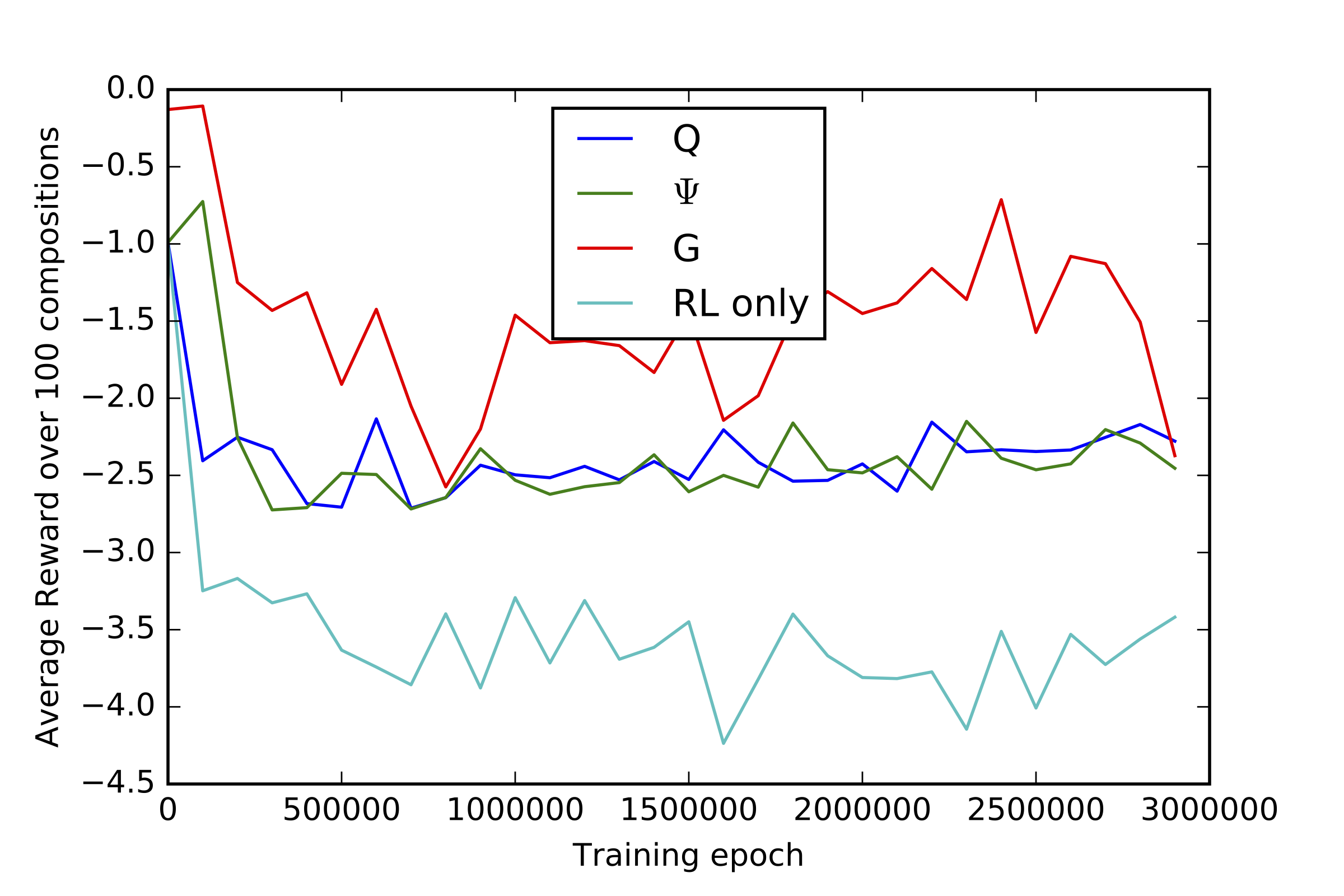
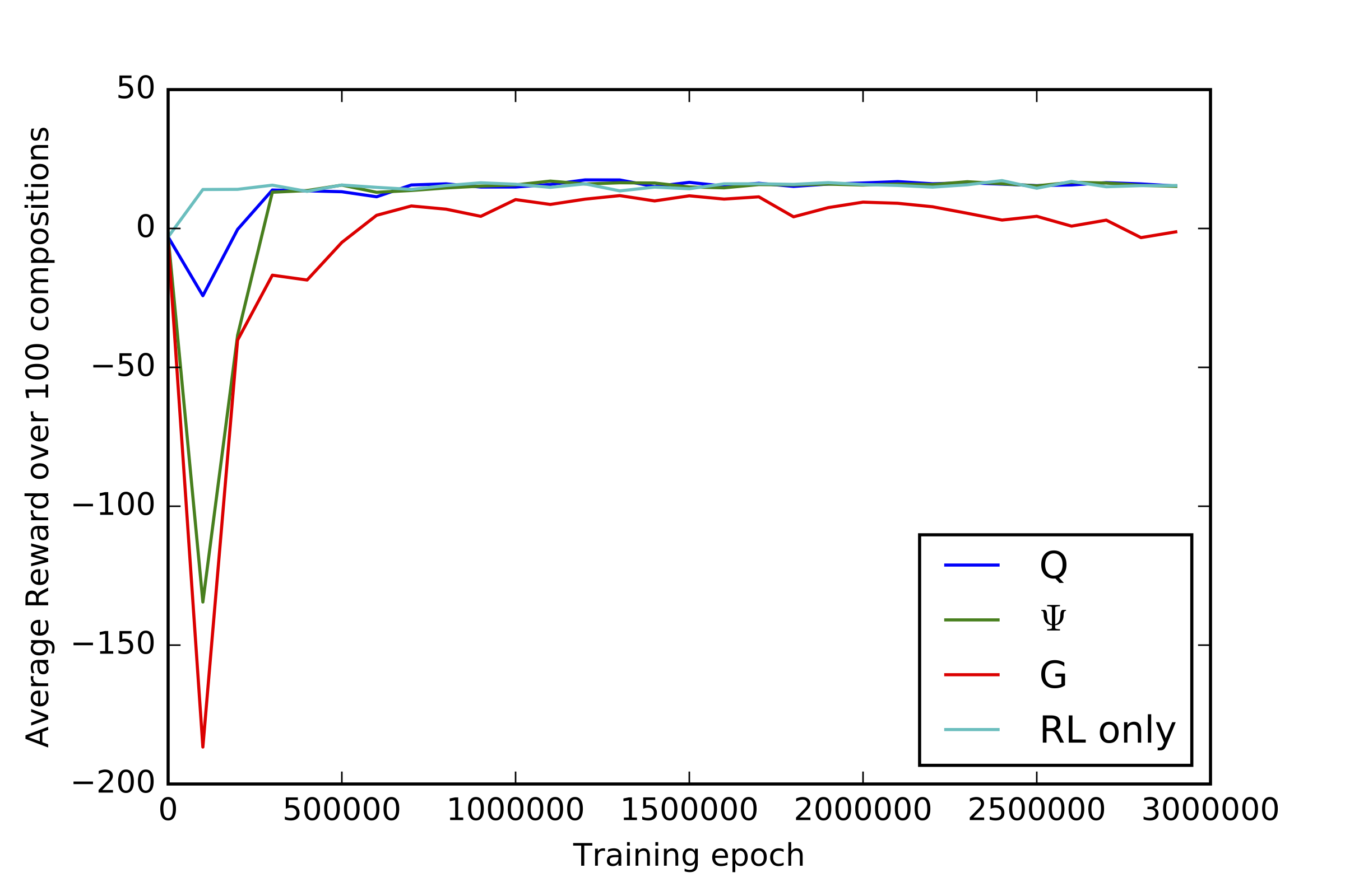
These results show that the targeted behaviors have significantly improved in the RL models as compared to the original Note RNN. But how do we know that learning these rules didn’t cause the models to forget what they learned from data? The figures below plot the rewards received by each model over time, broken down into the \(\log p(a\)|\(s)\) rewards from the Note RNN (on the left), and the music theory rewards \(r_{MT}\) (on the right). Each model is compared to a baseline RL only model that was trained using only the music theory rewards, and no information about the data probabilities. We see that compared to the RL only model, the RL Tuner models maintain much higher \(\log p(a\)|\(s)\), while still learning the music theory rewards.
 |
 |
|---|---|
| Note RNN rewards | Music theory rewards |
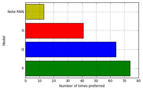
Even so, it’s not clear that learning this somewhat arbitrary set of music theory rules will lead to better sounding compositions. To find out whether the models have improved over the original Note RNN, we asked Mechanical Turk workers to rate which of two randomly selected compositions they preferred. The figure below shows the number of times a composition from each model was selected as the winner. All three RL Tuner models significantly outperformed the Note RNN, \(p<.001\). In addition, both the \(\Psi\) and \(Q\) models were statistically significantly better than the \(G\) model, although not significantly different from each other.
But you don’t need to take our word for it! The compositions used in the study are all available here - please check them out! Below, you can listen to a composition from each model. In the top row are compositions from the Note RNN and \(G\); in the bottom row are \(\Psi\) and \(Q\). You can see that the Note RNN plays the same note repeatedly, while the RL Tuner models sound much more varied and interesting. The \(\Psi\) and \(Q\) are best at playing within the music theory contraints, staying firmly in key and frequently choosing more harmonious interval steps. Still, we can tell that the models have retained information about the training songs. The \(Q\) sample ends with a riff that sounds very familiar!
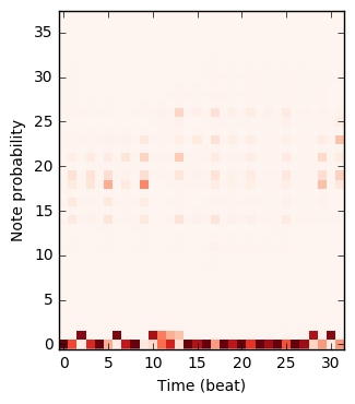
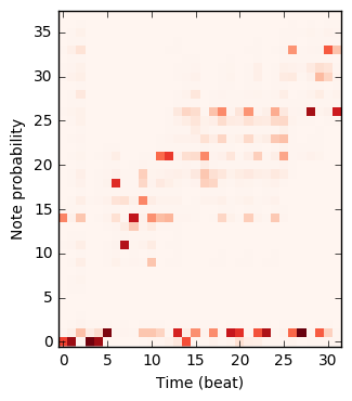
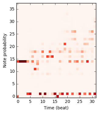
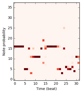
The figure below plots how the probability that the models place on each note changes during the composition. Note that 0 corresponds to the note off event, and 1 corresponds to no event; these are used for rests and holding notes.
 |
 |
 |
 |
|---|---|---|---|
| Note RNN | Q | \(\Psi\) | G |
Summary
In conclusion, we’ve demonstrated a technique for using RL to refine or tune (*pun intended*) an RNN trained on data. Although some researchers may prefer to train models end-to-end on data, this approach is limited by the quality of the data that can be collected. When the data contains hidden biases, this approach can really be problematic.
We hope you’ve enjoyed this post. If you’re interested in trying out the RL Tuner model for yourself, please check out the README file on the Magenta github.
Acknowledgements
This work was done in collaboration with Shane Gu, Richard E. Turner, and Douglas Eck. Many thanks also go to my wonderful collaborators on the Magenta team in Google Brain, and in particular Curtis (Fjord) Hawthorne and Kyle Kastner (for his knowledgeable insights and handy spectrogram-movie-producing code).