Waybackprop

TL;DR

I review (with animations!) backprop and truncated backprop through time (TBPTT), and introduce a multi-scale adaptation of TBPTT to hierarchical recurrent neural networks that has logarithmic space complexity. I wished to use this to study long-term dependencies, but the implementation got too complicated and kind of collapsed under its own weight. Finally, I lay out some reasons why long-term dependencies are difficult to deal with, going above and beyond the well-studied sort of gradient vanishing that is due to system dynamics.

Introduction

Last summer at Magenta, I took on a somewhat ambitious project. Whereas most of Magenta was working on the symbolic level (scores, MIDI, pianorolls), I felt that this left out several important aspects of music, such as timbre and phrasing. Instead, I decided to work on a generative model of real audio.

Audio is extremely high-dimensional. Even at a coarse sampling frequency of 11kHz, modeling one second of audio means modeling a joint distribution over 11000 variables. Moreover, audio in the form of a PCM stream (or, as Doug Eck likes to say, speaker cone positions) doesn’t respond well to downsampling. Time-frequency representations like (Short-Time) Fourier Transforms and Constant-Q are much nicer, but are really only used for information extraction and not for synthesis. The phase component is notoriously difficult to synthesize and usually thrown away even for purposes of information extraction. Although there exist invertible time-frequency representations, they are practically only one-way streets due to the phase.

Generative modeling is hard by itself, too. Consider images. It’s easy enough to, say, train an autoencoder to reconstruct images; that is, to minimize the Euclidean distance between its input and its output. But you’ll find that the images it produces are blurry because the model just learns to hedge its bets. When used as a loss function, Euclidean distance teaches the model that when it isn’t sure what to produce, it can get partial credit by just pixelwise averaging all candidate reconstructions.

The blurring issue is particularly apparent in the domain of images, but is a general characteristic of models trained to place high probability on training examples (i.e. maximum-likelihood). These models are punished harshly for putting low probability on even a single training data point, and as a result they spread their probability widely, producing generative distributions with high entropy. There is no counteracting incentive not to place probability on regions that don’t correspond to natural images.

Generative Adversarial Networks do have this counteracting incentive. GANs are trained not to produce particular outputs, but to match their generative distribution to the distribution that the training data came from, in such a way that an adversarial discriminator can’t tell generated examples from training examples. Unfortunately, the adversarial training process is very unstable; GANs are currently unreliable.

Under a maximum-likelihood objective, it is very difficult to get a model to focus on individual modes. Euclidean distance exacerbates this; it corresponds to treating the output of the model as the mean of a unimodal Gaussian with identity covariance. To encourage the model to break down the generative distribution into modes, it has recently become popular to quantize real-valued outputs and use a softmax output with cross-entropy loss instead. Although it feels wrong, the softmax approach is nice because it allows the model to represent arbitrarily shaped distributions.

Furthermore, modeling high-dimensional distributions becomes dramatically easier when the joint probability is broken up into autoregressive factors. There are many ways to do this. For sequences, chronological factorization is obvious and popular, in which the problem of modeling \(p(x_1, x_2 \ldots x_n)\) is broken up into the subproblems of modeling \(p(x_1), p(x_2 \mid x_1), p(x_3 \mid x_2, x_1)\) and \(p(x_n \mid x_{n-1} \ldots x_2, x_1)\). In order to be able to generalize to longer sequences we assume the conditional distributions are all equal, i.e. there is some stationary conditional distribution \(p(x_i \mid x_{<i})\) that we will model instead.

Autoregressive models are trained and evaluated by teacher-forcing, meaning the model receives as input the true values of the variables being conditioned on. During generation, however, these variables are not known, and the model conditions on its own best predictions of their values. This difference between training/evaluation and generation is a known source of trouble: the model only ever learns one-step transitions, and never learns to deal with its own errors. At generation time it can easily run off the tracks.

In the end, I went with an autoregressive recurrent neural network running on speaker cone positions. Recurrent neural networks are especially tough to apply to big data, but I had an idea I wanted to try out. But first, some background.

Backpropagation & memory use

To train a neural network, we typically run the model forward to compute its activations and output, and then work backwards to compute the gradient of the loss according to the chain rule of differentiation. While it is possible to accumulate the gradient going forward, working backwards is much more efficient as it involves smaller tensors and allows reuse of intermediate results. This is the backpropagation algorithm (pick your citation).

The value of the gradient depends on the activations of the neural network. Since we compute it backward, we need access to them in reverse order, starting from the last layer. However, computing the activations of the last layer involves computing the activations of all layers before it. Recomputing these intermediates as we work backwards takes \(O(n^2)\) time and \(O(1)\) space (where \(n\) is the number of layers). We might as well compute the activations in one forward pass and store them in memory for the backward pass, at the cost of \(O(n)\) time and \(O(n)\) space. Alternatively, we can checkpoint: store some activations and recompute others, at costs anywhere in between \(O(1)\) and \(O(n)\). See Dauvergne & Hascöet 2006 for an overview of checkpointing, and Chen et al. 2016 and Gruslys et al. 2016 for recent applications in deep learning.

Frameworks such as Theano and Tensorflow provide a symbolic differentiation operator, which takes a computation graph that runs the model forward and returns a new computation graph that runs backward to compute the gradient. The structure of the backward graph will reflect the reverse-order dependency on the activations. The framework will typically avoid the recomputation and choose to store the activations in GPU memory.

Truncated backpropagation through time

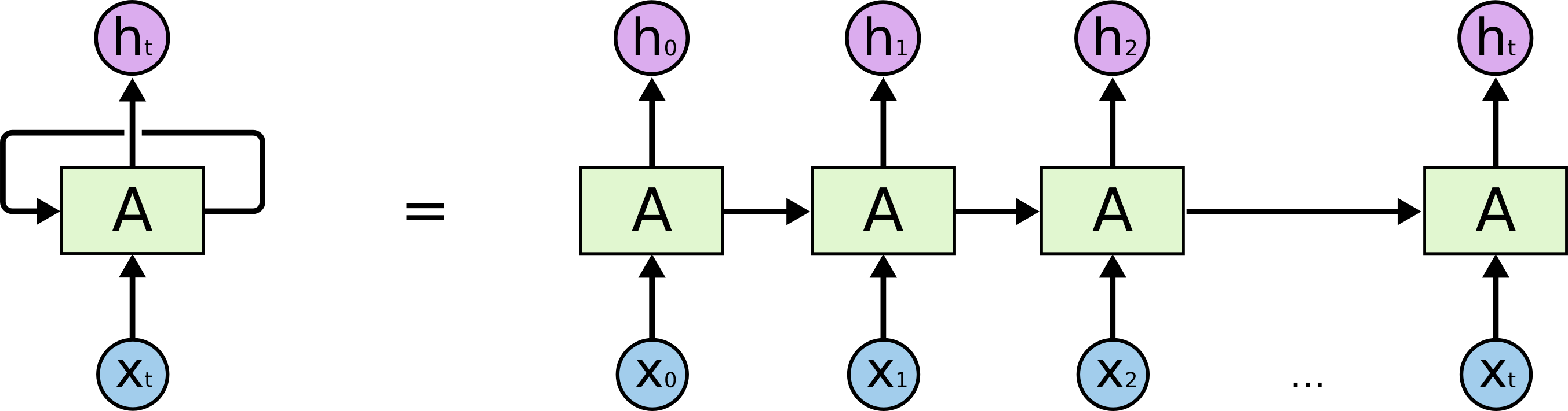
Backpropagation is easily adapted to recurrent neural networks by “unrolling” them, treating successive timesteps as if they were successive layers. This is backpropagation through time. Everything discussed in the previous section carries over to unrolled recurrent neural networks, where each state transition is treated as if it were a feedforward layer.

For autoregressive recurrent neural networks, we ideally want to run the model over one long sequence \(x\) of examples \(x_i \mid x_{<i}\). Examples of autoregressive tasks are language modeling tasks such as Penn Treebank (Marcus et al. 1993) and Wikipedia (Mahoney 2006), where the model processes a sequence of characters or words one at a time and at each step predicts the next character/word. However, because of the \(O(n)\) growth of memory usage, it is not feasible to compute gradient all the way back to the beginning of the sequence. Instead, it is customary to put a hard limit on the number of steps to run backwards. In practice this is implemented by slicing the long sequence into shorter subsequences and carrying over the model’s hidden state from one subsequence to the next. Typical subsequence length is anywhere from 50 to 1000 and is chosen to trade off minibatch size, number of hidden units and backpropagation length.

The following animation shows a gradient computation graph for a two-layer recurrent neural network:

Both the forward and the backward graph are shown, as well as the connections between them. Blue nodes represent hidden states, and the corresponding red node represents the gradient of the loss with respect to the hidden state. The loss node is shown in yellow at the far right. Inputs, outputs and parameters are omitted for simplicity. Computing the gradient with respect to the parameters is straightforward given the gradients with respect to the hidden states.

The animation shows the computation of nodes’ values over time. Each node is computed as soon as its dependencies are available. Note that while this ordering is logically valid, due to practical concerns it may not correspond to the actual ordering implemented in symbolic computation packages such as Theano and Tensorflow.

Truncated backpropagation through time conceptually looks like this:

This animation shows not just the order in which values are computed and stored, but also when they are forgotten. Each value is stored until each node that depends on it has been computed.

Repeatedly running the model forward and backing it up again seems like a silly thing to do. Indeed online methods for training recurrent neural networks are an active area of research, see e.g. Ollivier et al. 2015.

Waybackprop

Last summer, I worked on a recurrent generative model of music on the level of PCM-encoded acoustic signals. A major challenge in this setup is the extreme temporal resolution – it takes about ten thousand numbers to describe one second of sound. Clearly, if our model is to learn anything about the long-term structure of musical waveforms, we will have to train it on sequences longer than just a fraction of a second.

To do so, I developed a class of recurrent architectures that allow dramatically reduced space complexity through creative use of truncated backpropagation. The basic architecture is a Clockwork RNN (Koutník et al. 2014): a multi-layer recurrent structure where the bottom layer runs at the frequency of the data, and higher layers run on slower time scales.

Intuitively, you can think of the layers as being responsible for capturing increasingly coarse musical structure, from spikes and sines at the bottom to notes, phrases and chord changes at the top. Hierarchical architectures like these have been around for a long time (Schmidhuber 1992, El Hihi & Bengio 1995) and are currently being revisited (Koutník et al. 2014, Chung et al. 2016).

What’s new is the application of truncated backpropagation on all levels of the model. Rather than having a single cutoff point for all layers, each layer has its own, thus allowing the truncation to be tailored to the frequency of the layer. In particular, by backpropagating over much shorter distances at the bottom and much longer distances at the top, many fewer hidden states need to be kept in memory. The memory thus saved can be used not just to backprop longer, but also to backprop through models with much larger hidden representations.

Here’s an example:

In the example above, the bottom layer updates at every step, the middle layer updates every three steps, and the top layer updates every nine steps. By truncating the backprop at the end of each layer’s period (i.e. before its state propagates upward), the backward graph is greatly reduced in size. In particular, it doesn’t depend on all those states on the bottom which don’t convey long-term information anyway. Consequently, the storage requirements are \(O(\log T)\) where \(T\) is the number of time steps, as compared to the usual \(O(T)\). That is, given a fixed memory budget, we can get orders of magnitude increases in the length of dependencies captured by the backpropagated gradient.

Implementation

If the number of time steps is known at graph construction time, the implementation of waybackprop is simple:

while t < T:
  for i, stride in reversed(enumerate(layer_strides)):
    is_due = t % stride == 0
    if is_due:
      # truncate gradient on state below, before it is used upward or rightward
      states[i - 1] = tf.stop_gradient(states[i - 1])
      # update state based on states above, to the left and below
      states[i] = cells[i](states[i - 1:i + 1])
  t += 1

Theano and Tensorflow both come with a gradient truncation operator (theano.gradient.disconnected_grad and tf.stop_gradient, respectively). This operator is used during construction of the forward computation graph, to indicate nodes that should be considered constant for the purposes of differentiation. During construction of the backward graph, the differentiation operator stumbles upon these nodes and knows not to recurse on them.

In a symbolic loop (theano.scan, tf.while_loop) however, things get hairy. These loops are specified using functions that compute subgraphs which are then repeatedly evaluated:

def body(t, states):
  for i, stride in reversed(enumerate(layer_strides)):
    is_due = t % stride == 0
    states[i - 1] = tf.cond(is_due,
                            partial(tf.stop_gradient, states[i - 1]),
                            partial(tf.identity, states[i - 1]))
    states[i]     = tf.cond(is_due,
                            partial(cell[i], states[max(0, i - 1):i + 1]),
                            partial(tf.identity, states[i]))
  return (t + 1, states))
t, states = tf.while_loop(lambda t: t < T, body, loops_vars=[t, states])

The gradient through a symbolic loop will itself take the form of a symbolic loop, and hence share graph structure across loop iterations. This means we cannot use gradient truncation to arbitrarily prune the backward graph.

Ultimately, I ended up partially unrolling the symbolic loop, moving the upper layers into a static outer loop. This creates many shorter symbolic loops, allowing approximation of the desired backward graph structure by truncating on a coarser level, between the symbolic loops. In the limit of unrolling all layers, the situation is equivalent to a static loop.

Of course, the problem with static loops is graph size. With partial unrolling, my computation graph contains millions of nodes. Tensorflow takes 200GBs of CPU memory to handle it, and all of our debugging tools break down. After leaving Google, I no longer have the resources to run this model.

Discussion

Whenever I was able to run the model, the results were negative. I will not bore you with the details, but it seems that backpropagating gradient over longer distances (as long as a million steps) does not help for autoregressive modeling of audio and character-level text. Now, like any self-respecting researcher who has trouble letting go of cherished ideas in the face of disconfirming evidence, I believe that waybackprop should be helpful in principle, and that the memory issue is only one of many barriers on the road to successful modeling of long-term dependencies:

• As is well known, gradients vanish. Both the forward pass and the backward pass of recurrent neural networks implement dynamical systems which may be chaotic. In particular, gradients may vanish or explode based on the singular values of the recurrent transition matrix. Much has been written about this; see e.g. Hochreiter 1991, Bengio et al. 1994, Gers 2001, Pascanu et al. 2012, Martens 2016 and many of the other references in this document. Clearly, if we are to model long-term dependencies, at the very least the learning signal must reach far enough back!
• Our tasks are dominated by short-term dependencies: language modeling benchmarks such as enwik9 or Penn Treebank (Mikolov et al. 2012) appear to be “one long sequence” but actually consist of concatenations of short sequences with no dependence between them. Even truly long waveform has very strong local structure that must be modeled.
• Moreover, our loss is dominated by short-term dependencies: we only ever ask the model to predict one step ahead. In smooth signals such as audio this puts a strong emphasis on modeling high-frequency (i.e. short-term) behavior, since the low frequencies have much less of an effect on the waveform amplitude from one sample to the next. In fact if the sampling frequency is high enough, a good way to get low teacher-forcing loss on smooth signals such as audio is to predict that \(x_i = x_{i-1}\), that is, the signal is constant. This is a terrible generative model of audio as it will only ever generate a constant signal. But the loss is good. Clearly RNNs learn much more interesting functions, but they do so despite being disproportionately punished for getting the short-term dependencies wrong.
• Long-term dependencies are abstract and subtle. In character-level language modeling, two characters three sentences apart are uncorrelated. Likewise, two speaker cone positions three milliseconds apart have no dependency between them. Instead, the dependencies happen on a very abstract level, which the model must have the capacity to represent. If the model does not have the right representation, long-term gradients will vanish for reasons nothing to do with the singular values of the recurrent transition function.
• Given the previous point, maximum likelihood losses on surface-level features (e.g. L2 on pixels, or cross-entropy on quantized waveforms) puts an additional emphasis on details over big picture. We present the model with a partial example and ask it to complete it in a particular way. Of course, many completions are possible, even many completions that are equivalent on an abstract level. But we only have one completion in our dataset, and the model had better give us that one or else.

These insights are not novel at all, but they didn’t feel concrete until I personally banged my head against them. I believe it would be valuable to design experiments that tease these obstacles apart so that we can get an idea of their relative importance and address them in isolation.

As for audio, I never obtained decent samples except when overfitting to a single short example. I have become skeptical of the quantized waveform representation. Replacing a real-valued mixture-of-Gaussians output model with a softmax in many ways eases optimization and avoids failure modes where the model tries to cover multiple modes with a single mode. However it makes it awkward to represent the signal as a sum of signals, in other words to exploit the superposition principle. On the other hand, WaveNet (Van Den Oord et al. 2016) and SampleRNN (Mehri et al. 2016) use the same representation, successfully.

Acknowledgements

I’m grateful to the entire Magenta team but particularly my hosts Fred Bertsch and Douglas Eck, and co-conspirators Anna Huang, Natasha Jaques and Kyle Kastner. Further thanks go to Brain members George Dahl, Eugene Brevdo and David Bieber for helpful discussions. Finally, I thank Aaron Courville for advice, and Alex Lamb for proofreading.

References

Bengio et al. 1994. Learning Long-Term Dependencies with Gradient Descent is Difficult
Chen et al. 2016. Training Deep Nets with Sublinear Memory Cost
Chung et al. 2016. Hierarchical Multiscale Recurrent Neural Networks
Dauvergne & Hascöet 2006. The Data-Flow Equations of Checkpointing in reverse Automatic Differentiation
El Hihi & Bengio 1995. Hierarchical Recurrent Neural Networks for Long-Term Dependencies
Gers 2001. Long Short-Term Memory in Recurrent Neural Networks
Gruslys et al. 2016. Memory-Efficient Backpropagation Through Time
Hochreiter 1991. Untersuchungen zu dynamischen neuronalen Netzen
Koutník et al. 2014. A Clockwork RNN
Mahoney 2006. Large Text Compression Benchmark
Marcus et al. 1993. Building a large annotated corpus of English: the Penn Treebank
Martens 2016. Second-order Optimization for Neural Networks
Mehri et al. 2016. SampleRNN: An Unconditional End-to-End Neural Audio Generation Model
Mikolov et al. 2012. Subword Language Modeling with Neural Networks
Ollivier et al. 2015. Training recurrent networks online without backtracking
Pascanu et al. 2012. On the difficulty of training Recurrent Neural Networks
Schmidhuber 1992. Learning Complex, Extended Sequences Using the Principle of History Compression
Van Den Oord et al. 2016. WaveNet: A Generative Model for Raw Audio