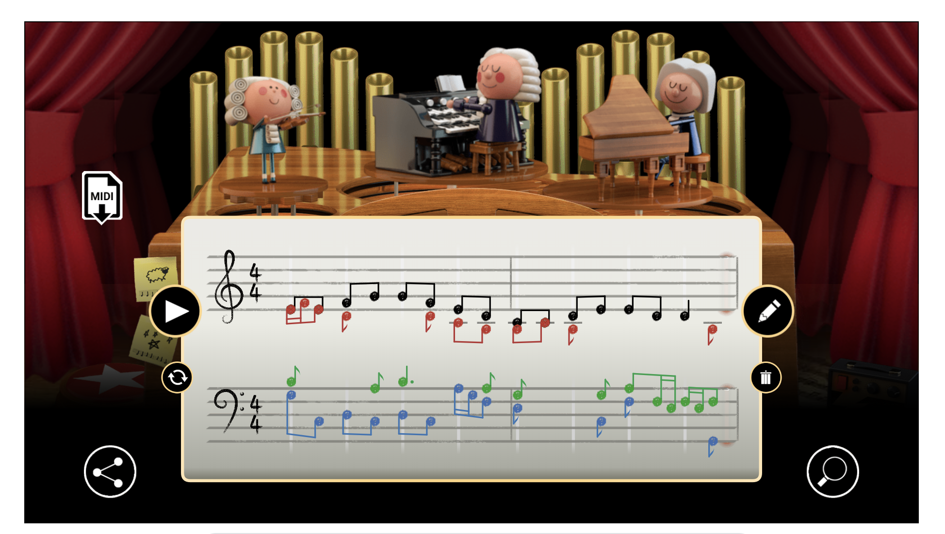
Have you seen today’s Doodle? Join us to celebrate J.S. Bach’s 334th birthday with the first AI-powered Google Doodle. You can create your own melody, and the machine learning model will harmonize it in Bach’s style.

In this blog post, we introduce Coconet, the machine learning model behind the Doodle. We started working on this model 3 years ago, the summer when Magenta launched. At the time we were using machine learning (ML) only to generate melodies. It’s hard to write a good melody, let alone counterpoint, where multiple melodic lines need to sound good together. Like every music student, we turned to Bach for help! Using a dataset of 306 chorale harmonizations by Bach, we were able to train machine learning models to generate polyphonic music in the style of Bach.

Coconet is trained to restore Bach’s music from fragments: we take a piece from Bach, randomly erase some notes, and ask the model to guess the missing notes from context. The result is a versatile model of counterpoint that accepts arbitrarily incomplete scores as input and works out complete scores. This setup covers a wide range of musical tasks, such as harmonizing melodies, creating smooth transitions, rewriting and elaborating existing music, and composing from scratch.

Whereas traditional models generate notes in chronological order from beginning to end, Coconet can start anywhere and develop the material in any order. This flexibility makes it attractive as a tool to support the compositional process. One way a musician might incorporate this into their workflow is to repeatedly let Coconet fill out the score, each time keeping the good stuff and erasing the rest. In fact, this is how Coconet works internally: it produces material in a loop, repeatedly rewriting and erasing its own work. It starts with rough ideas, and then goes back and forth to work out details and tweak the material into a coherent whole.

Is this rewriting really necessary? When we showed Coconet to a musician friend of ours, he got very excited and wanted to take it for a spin. After several weeks of anticipation, we received from him a carefully crafted MIDI file containing… the melody from Ode to Joy. Except that he had modified the ending to abruptly modulate upwards in an attempt to derail Coconet. Thanks to its rewriting process, Coconet was able to find a harmonization that accommodates the twist:

The animation below shows a visualization of this rewriting process. Read on to learn more about what these animations mean and how the model works.

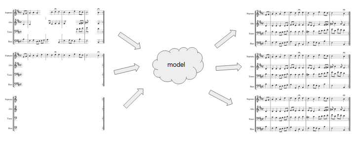
We show two examples of Coconet harmonizing melodies from Bach chorales that were not included in the training set. On the left are the original chorale melodies and on the right are Coconet’s harmonizations.

The two samples below are Coconet composing from scratch.

We’ve also built an expanded interface, called Coucou, that allows more general interaction with Coconet. It enables a new type of collaborative composition with AI, where you can iteratively improve a musical piece by erasing parts that are unsatisfying and asking the model to infill again. You can click infill repeatedly to get different variations. Try out the examples below or start by splashing random notes on a page. You can also build your own interfaces using the JavaScript implementation now available in Magenta.js.

If you’re new to writing music, don’t worry: the model will try its best to make the result sound like Bach. Plus you can always try again or ask the model to try again! For musicians, we hope this model can help you prototype ideas more quickly and explore more variations, or find inspiration in a motif, an unexpected turn in harmony or rhythm. We’re excited to see what you come up with and hope you have fun writing music with Coconet! Keep reading to learn more details about how this model works and a technical explanation of why it works.

How does it work?

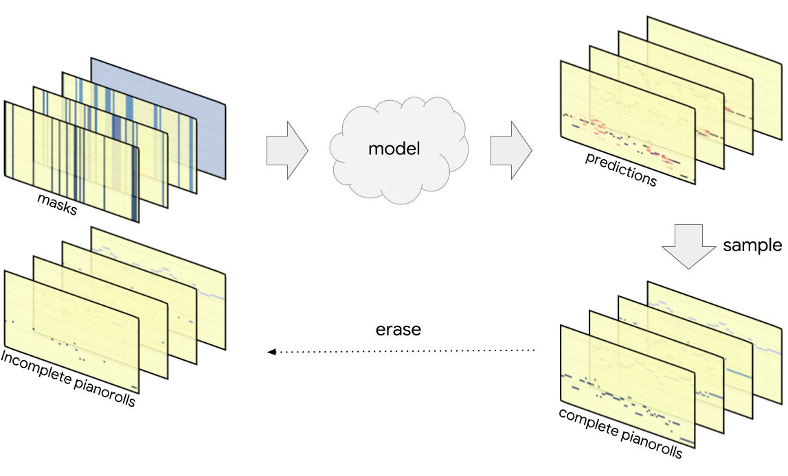
Coconet takes incomplete musical scores and fills in the missing material. To train it, we take an example from the Bach chorales dataset of four-part counterpoint, randomly erase some notes, and ask the model to reconstruct the erased notes. The difference between Bach’s composition and Coconet’s fabrication gives us a learning signal by which we can train our model.

By erasing notes randomly, we hope to obtain a model that can handle arbitrarily incomplete input. Below, in the “Why does it work?” section, we show an interesting interpretation of this training procedure as equivalent to training many models at once, each one applicable in a different scenario.

For our purposes, “musical scores” are three-dimensional objects. The Bach chorales are written for four voices, soprano (S), alto (A), tenor (T) and bass (B). The music for each voice is represented in pianoroll: a two-dimensional array with (discretized) time extending horizontally and pitches laid out vertically. We assumed each voice sings exactly one pitch at any given time. Thus ordinarily for each voice, at each point in time, we have a one-hot pitch vector whose elements are all zero except for a single one indicating the pitch being sung. In the presence of uncertainty (e.g., in the model output) this pitch vector will contain a categorical probability distribution over the pitches.

(The one-hot pitch assumption can be relaxed to multi-hot in order to incorporate silences and polyphonic instruments, although this comes at a cost of about a fifty-fold increase in the number of variables.)

We treat this stack of pianorolls as a convolutional featuremap, with time and pitch forming the two-dimensional convolutional space, and each voice providing a channel. As the scores we will be feeding into the model are incomplete, we supply one additional channel per voice with a mask: binary values indicating at each point in time whether the pitch for that voice is known. Thus what goes into the model is an eight-channel featuremap.

The model is a fairly straightforward convolutional neural network with batch normalization and residual connections. For the doodle, which runs the model in the browser using a Tensorflow.js implementation, we were able to speed up the computations by switching to depthwise-separable convolutions. These differ from regular convolutions in that they separate the convolution across the spatial axes and the mixing across the channel axis. They require fewer parameters and are more amenable to acceleration in the browser. We achieved a further speedup by reducing the number of layers in the model without suffering a loss of performance, thanks to dilated convolutions.

What comes out of the model is again a stack of pianorolls, one per voice, but this time containing probability distributions over the pitches of the erased notes. The model uses the notes that were given to try to figure out the notes that were erased, resulting in a categorical distribution over the pitch being sung by each voice at each point in time.

We train the model to assign high probability to the true pitches. This pushes it to understand the musical implications of the incomplete score it was given – what key are we in, what chord are we singing here, where are we going, and where did we come from?

Once the model is trained, we have several ways of extracting music from the probability distributions produced by the model. We can sample each of the pitches simultaneously according to its distribution. However, as discussed at length below under “Why does it work?”, this would not account for interactions between the pitches being sampled. Often, determining one of the pitches would change the distributions for the other pitches.

One way of accounting for these interactions would be to sample one of the pitches, add it to the incomplete score, and pass the result through the model again to recompute the distributions for the remaining pitches. By repeating this process until all pitches have been determined, we complete the score while taking all interactions into account. This sequential sampling procedure expects the model to be able to accurately determine the unknown pitches one by one. This strong assumption often leads these processes off the rails when the model gets increasingly confused by its own creation.

We instead use a more robust procedure: we treat the model’s output as a rough draft, which we gradually refine by repeated rewrites. Specifically, we sample all of the pitches simultaneously, obtaining a complete (but typically nonsensical) score, which is then partially erased and passed into the model again, after which the process repeats. Over time, we erase and rewrite fewer and fewer notes, enabling the process to settle on a coherent result.

Why does it work?

In this section, we lay out a more technical understanding of Coconet as an ensemble of autoregressive structures that includes the familiar chronological structure common in sequence models. To simplify the presentation, we will consider a toy example of modeling a sequence of three variables, \(x_1\), \(x_2\) and \(x_3\). Concretely, this could be a three-note melody, or a three-tone chord, with each variable taking a pitch as its value. The problem of modeling the sequence of \(x_1\), \(x_2\), \(x_3\) is then the problem of representing and learning the joint probability distribution \(p(x_1, x_2, x_3)\) of how likely is a given sequence \(x_1\), \(x_2\), \(x_3\) to occur in natural data?

This is a hard problem as it is not enough to model the independent (marginal) distributions \(p(x_1)\), \(p(x_2)\), \(p(x_3)\) because the variables interact. For each possible value of \(x_1\), there are conditional distributions \(p(x_2\vert x_1)\), \(p(x_3\vert x_1)\) on the other variables that depend on the value of \(x_1\) (just as the second note in a three-note melody will depend on the first note, and the second tone in a three-tone chord will depend on the first tone). If we have models of both \(p(x_1)\) and \(p(x_2\vert x_1)\), we can compose them to obtain a model of \(p(x_1, x_2) = p(x_1) p(x_2\vert x_1)\). If we also have a model of \(p(x_3\vert x_1, x_2)\), we can compose all three to obtain a model of the desired joint distribution \(p(x_1, x_2, x_3) = p(x_1) p(x_2\vert x_1) p(x_3\vert x_1, x_2)\).

This is one example of an autoregressive factorization of the joint probability distribution: the hard-to-handle function \(p(x_1, x_2, x_3)\) is broken up into autoregressive factors \(p(x_1)\), \(p(x_2\vert x_1)\) and \(p(x_3\vert x_1, x_2)\).

Modeling one variable at a time

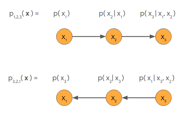
The above factorization is the most natural for sequence data, as it follows the order of the sequence. In the context of monophonic music (such as a melody), that means the distribution for each note is informed by the notes leading up to it. This gives us the forward ordering (1,2,3). Another natural factorization is to go backwards (3,2,1): establish the conclusion first, then work away from it. We can represent these graphically as follows:

More generally, there exists an autoregressive factorization for each possible ordering of the variables. In a problem with N variables, there are N! possible orderings. In our three-variable case, we can enumerate all six of them:

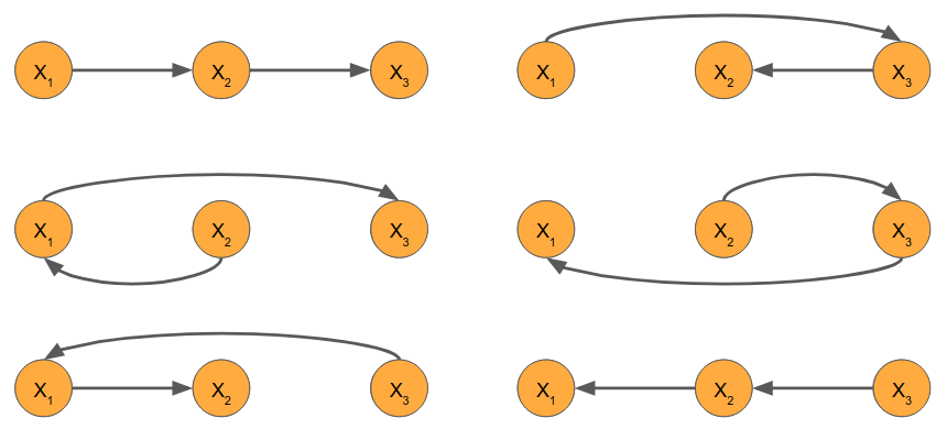
These all provide viable ways of modeling three-note melodies or three-tone chords. In theory, it makes no difference which ordering you choose. In practice, however, the choice of ordering determines the applicability of the model – you can’t play along in real time with a backwards model – and introduces an inductive bias that has strong and unintuitive effects on what the model learns. That is, in practice, models trained according to different factorizations end up learning different joint distributions.

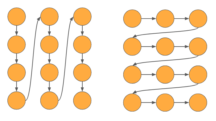
Polyphonic music consists of multiple simultaneous sequences – multiple instruments playing together. In this case there isn’t really a natural ordering of the variables, although there are two obvious ways in which to flatten the multiple sequences. They are shown below, with time running horizontally and instruments laid out vertically:

On the left, we have interleaved the instruments; the ordering is S, A, T, B, S, A, T, B etc. This ordering favors harmony: the model generates the music one chord at a time. On the right, we have concatenated the instrument parts, to give the ordering S, S, S, S, A, A, A, A etc. Now we favor melody, as the model generates one line after another. These two very different perspectives are actually a familiar source of tension in music theory.

No single ordering really works for us – we wish to be able to complete arbitrarily partial scores. A composer may give us only the beginning of a score, or only the end, or both the beginning and end but not the middle. Or one or more instruments may be missing. Or several instruments may be missing material at different measures. We cannot depend on any instrument coming before another, or any measure coming before any other. In fact, we need to be able to support any ordering!

Orderless modeling

As it turns out, our intuitively motivated training procedure based on inpainting has us covered. When we feed a partially erased score into the model, what comes out can be interpreted as conditionally independent distributions over the erased variables. Let us return to our example of the three-variable sequence \(x_1\), \(x_2\), \(x_3\). Suppose we erase \(x_2\) and \(x_3\); then the model observes \(x_1\) and produces conditional distributions on the values of \(x_2\) and \(x_3\).

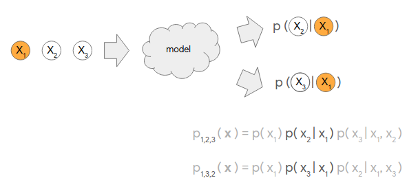
The conditional distributions \(p(x_2\vert x_1)\) and \(p(x_3\vert x_1)\) so obtained appear as factors in two of the six orderings of the three variables. In general, depending on which variables we erase, we can compute any conditional factor from any of the orderings. By composing such conditional factors, we can form a model corresponding to any desired ordering. Essentially, the inpainting model provides an ensemble of autoregressive models, one model for each possible ordering!

Moreover, we can train this ensemble much more efficiently than the naive approach of sampling an ordering and evaluating its conditional factors one by one. The key observation is that each conditional is shared among many orderings: even in our low-dimensional example, \(p(x_3\vert x_1,x_2)\) is shared by two orderings (1,2,3 and 2,1,3). Generally, all of these conditional distributions \(p(x_i\vert x_C)\) (where \(x_C\) is any subset of the variables not including \(x_i\)) are independent of the ordering of the variables that come before or after \(x_i\), which greatly reduces the number of distinct probability distributions we need to learn.

To train Coconet, then, we take a training example from our dataset, choose uniformly how many variables to erase, and choose uniformly the particular subset of variables to erase. We feed the partially erased score into the model (along with a mask indicating which variables were erased) and obtain a set of independent distributions over the values of the erased variables. We then compute the log-likelihoods of the true values and average across the erased variables, which corrects for a subtle scaling issue. This gives us the loss, which we minimize using backprop and stochastic gradient descent as usual.

We were not the first to discover this orderless interpretation of inpainting models. In 2014, Uria et al. proposed Orderless NADE, an orderless version of the Neural Autoregressive Distribution Estimator (NADE) that has exactly the same structure as our model. The difference between Coconet and Orderless NADE is in the process used to sample from the trained model.

Use Gibbs sampling to generate from multiple orderings

Although Orderless NADE learns an ensemble of orderings, the associated sampling procedure still effectively samples according to a single ordering. Specifically, Uria et al. proposed to uniformly choose an ordering, and then generate the variables one by one according to the chosen ordering. The music is still composed in a single pass, and no iterative improvement takes place.

Why might it be hard to write music in a single pass? Say we’re starting from an empty page, and have to write down our first note for a symphony, knowing we can not change it later. This is a tough decision: we have to account for all the possible futures we might be in and this note has to be right. Later on, as more notes are in place, we have more context to inform our decisions. What if we didn’t have to compose from scratch and could always have some context to work with.

And it turns out we can, by using Gibbs sampling! Gibbs sampling is a process that samples from a joint distribution by repeatedly resampling individual variables. We use it as a metaphor for repeatedly rewriting parts of a musical score. At every step, we erase parts of the score and let the model rewrite the erased parts. This way, the model always has some context to anchor to. Although the context is itself in flux and likely to be rewritten on later iterations, that’s okay: the model’s current decisions are not set in stone either. Gradually, the score settles into an internally consistent state.

The process just described is more accurately called blocked Gibbs sampling because we resample more than one variable at a time. If you were to visualize the probability distribution as a landscape, you would see peaks at probable configurations, separated by vast valleys of improbable configurations. Mass resampling helps explore the space of possibilities by taking large jumps, whereas resampling one variable at a time tends to settle on a nearby peak. Hence, we anneal the block size: we start by rewriting large portions of the score in order to explore the space, and we gradually rewrite less and less in order to settle on a plausible musical score.

Blocked Gibbs sampling raises the question of how to sample within the block: if \(x_1\) and \(x_2\) were erased, we can resample them from their proper joint \(p(x_1, x_2 \vert x_3)\) according to one of two orderings. However, this requires a pass through the model for each variable to be resampled, which rapidly becomes too slow when you do it repeatedly as part of a Gibbs process. In 2014, Yao et al. proposed to resample simultaneously from the independent distributions \(p(x_1 \vert x_3)\) and \(p(x_2 \vert x_3)\) produced by a single model evaluation. This works as long as we anneal the block size over time, so that eventually we are sampling one variable at a time conditioned on all the other variables, as in the basic Gibbs sampling algorithm. While Yao et al. thought of this as a faster approximation to the original Orderless NADE sampling procedure, in our paper we show empirically that for our use case it actually improves the quality of the samples.

Acknowledgements

This blog post is based on the Counterpoint by Convolution paper authored by Cheng-Zhi Anna Huang, Tim Cooijmans, Adam Roberts, Aaron Courville and Douglas Eck. The Tensorflow code from the research paper is available in Magenta GitHub.

@inproceedings{huang2017counterpoint,
 title={Counterpoint by Convolution},
 author={Huang, Cheng-Zhi Anna and Cooijmans, Tim and Roberts, Adam and Courville, Aaron and Eck, Douglas},
 booktitle = {International Society for Music Information Retrieval (ISMIR)},
 year={2017}
}

Special thanks to our friend Stefaan De Rycke for coming up with the tweaked Ode to Joy test for Coconet. Big thanks to James Wexler for implementing the Tensorflow.js version of Coconet for the Bach Doodle, and also Ann Yuan, Daniel Smilkov, Nikhil Thorat on Tensorflow.js and Pair Team. And a big shoutout to Jacob Howcroft, Leon Hong, Pedro Vergani, Rebecca Thomas, Jordan Thompson and others on the Doodle team for a delightful interactive ML experience!