In a previous post, we described the details of NSynth (Neural Audio Synthesis), a new approach to audio synthesis using neural networks. We hinted at further releases to enable you to make your own music with these technologies. Today, we’re excited to follow through on that promise by releasing a playable set of neural synthesizer instruments:

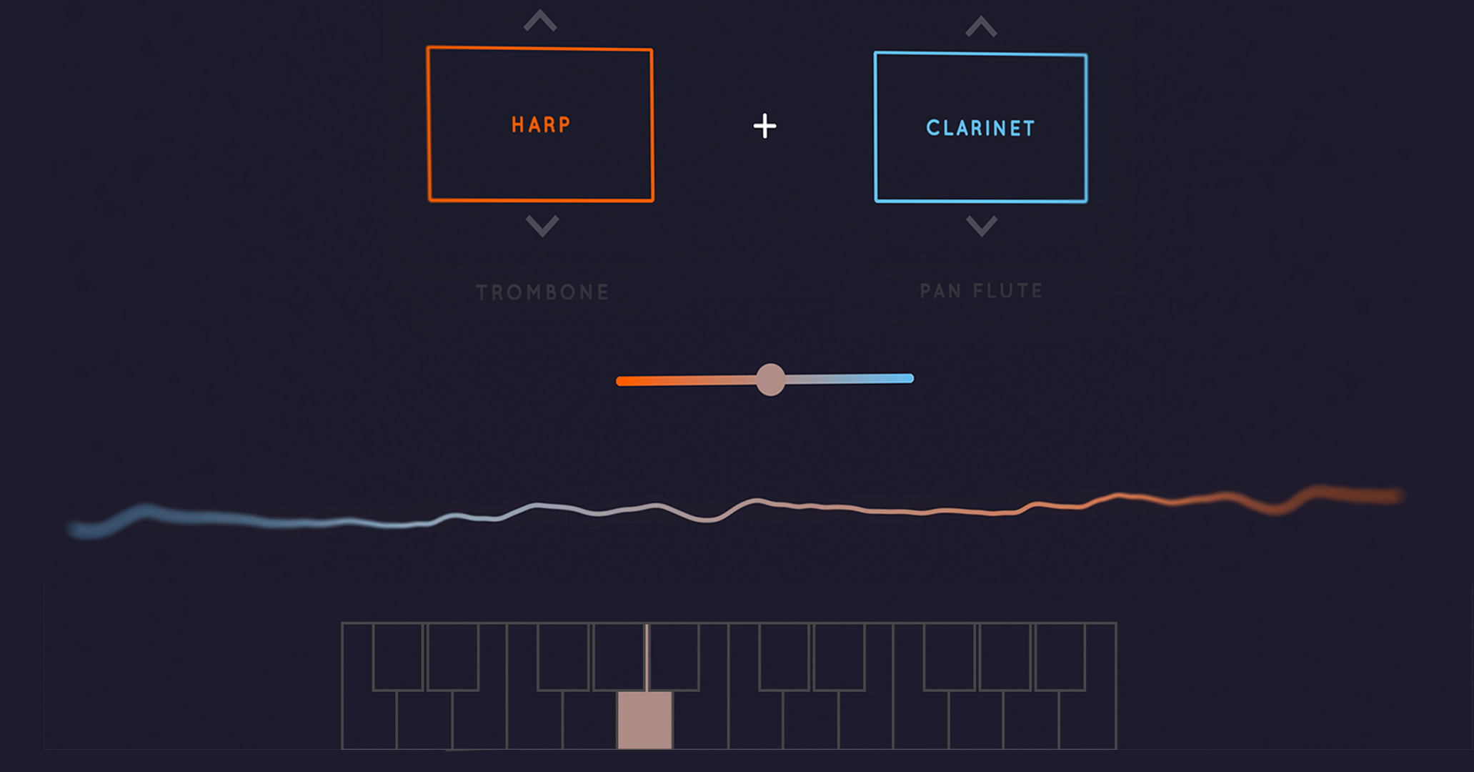
• An interactive AI Experiment made in collaboration with Google Creative Lab that lets you interpolate between pairs of instruments to create new sounds.

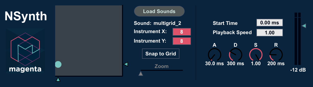
• A MaxForLive Device that integrates into both Max MSP and Ableton Live. It allows you to explore the space of NSynth sounds through an intuitive grid interface. [DOWNLOAD]

The goal of Magenta is not just to develop new generative algorithms, but to “close the creative loop”. We want to empower creators with tools built with machine learning that also inspire future research directions. Instead of using AI in the place of human creativity, we strive to infuse our tools with deeper understanding so that they are more intuitive and inspiring. We hope that these instruments are one small step in that direction, and we’re really excited to see what you make with them.

From Interpolation to Instrument

We also had a great time developing these instruments and wanted to share some of our process in making a creative musical tool out of a generative algorithm. As a quick reminder, the NSynth algorithm works by finding a compressed representation of sound (let’s call it “z”). In this simplified diagram, you can see that an encoder network transforms a sound into its z representation. A decoder network then converts it back into sound. The whole system is trained so that the reproduced sound is as similar as possible to the real sound. You can find more details in the original post and paper.

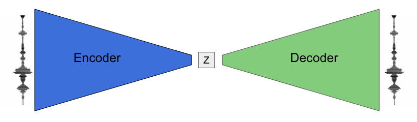
Since the network tries to reproduce the sounds as best it can, it maps similar sounds to similar z-representations¹. Normally, mixing the audio of two instruments creates a sound of the two instruments being played simultaneously. In contrast, mixing the z-representations and then decoding results in what sounds more like a single hybrid instrument.

Lines, Grids, and Multigrids

We designed our instruments around interpolating among different sounds and timbres. The Creative Lab Experiment demonstrates this clearly, allowing you to select pairs of instruments and dragging a slider to play all the gradations between the instruments.

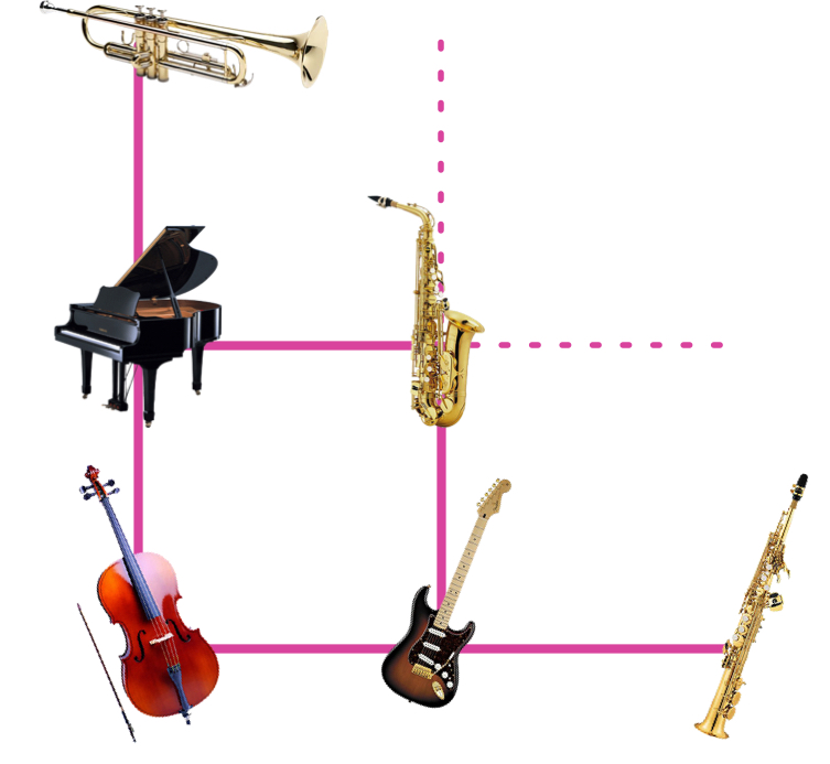
For the Ableton Live instrument, we positioned instruments at the corners of a square grid, allowing you to mix among all four. Even further, we tiled a bunch of these four instrument grids next to each other, creating a “multigrid”. This interface allows you to explore up to 64 different instruments by dragging across a single x-y pad. At every point, you are mixing the four nearest instruments.

Because the WaveNet decoder is computationally expensive, we had to do some clever tricks to make this experience run in real-time on a laptop. Rather than generating sounds on demand, we curated a set of original sounds ahead of time. We then synthesized all of their interpolated z-representations. To smooth out the transitions, we additionally mix the audio in real-time from the nearest sound on the grid. This is a classic case of trading off computation and memory.

We added a few more UI bells and whistles to make the instrument more fun and playable. In the video below, watch Jesse go through the process of setting up and playing the instrument in Ableton.

These designs are just one possible approach to neural audio synthesis, and we’re really excited to see what the community comes up with in exploring this new paradigm of audio generation.

Unique sound

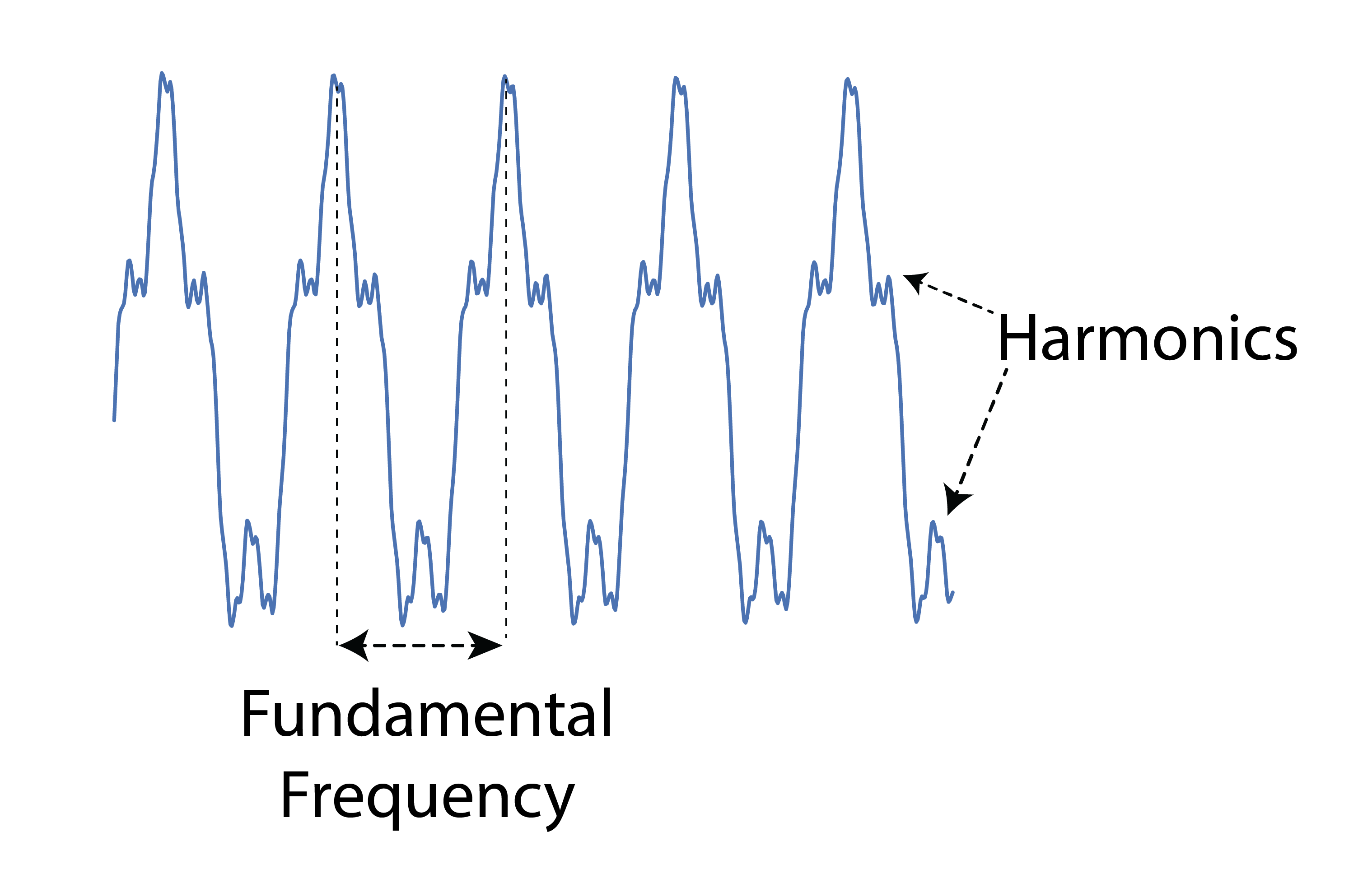
As you play around with these instruments, you’ll see that the algorithm does not exactly reproduce the sounds. First, for computational reasons, we work on mu-law encoded 8-bit 16kHz sound, which adds a gritty texture to the sounds. It’s also really interesting to listen to the ways in which the algorithm “fails” to fit the data. The fundamental frequency of a sound is given by the rate a waveform repeats, but the harmonic structure is given by the shape of the waveform that repeats.

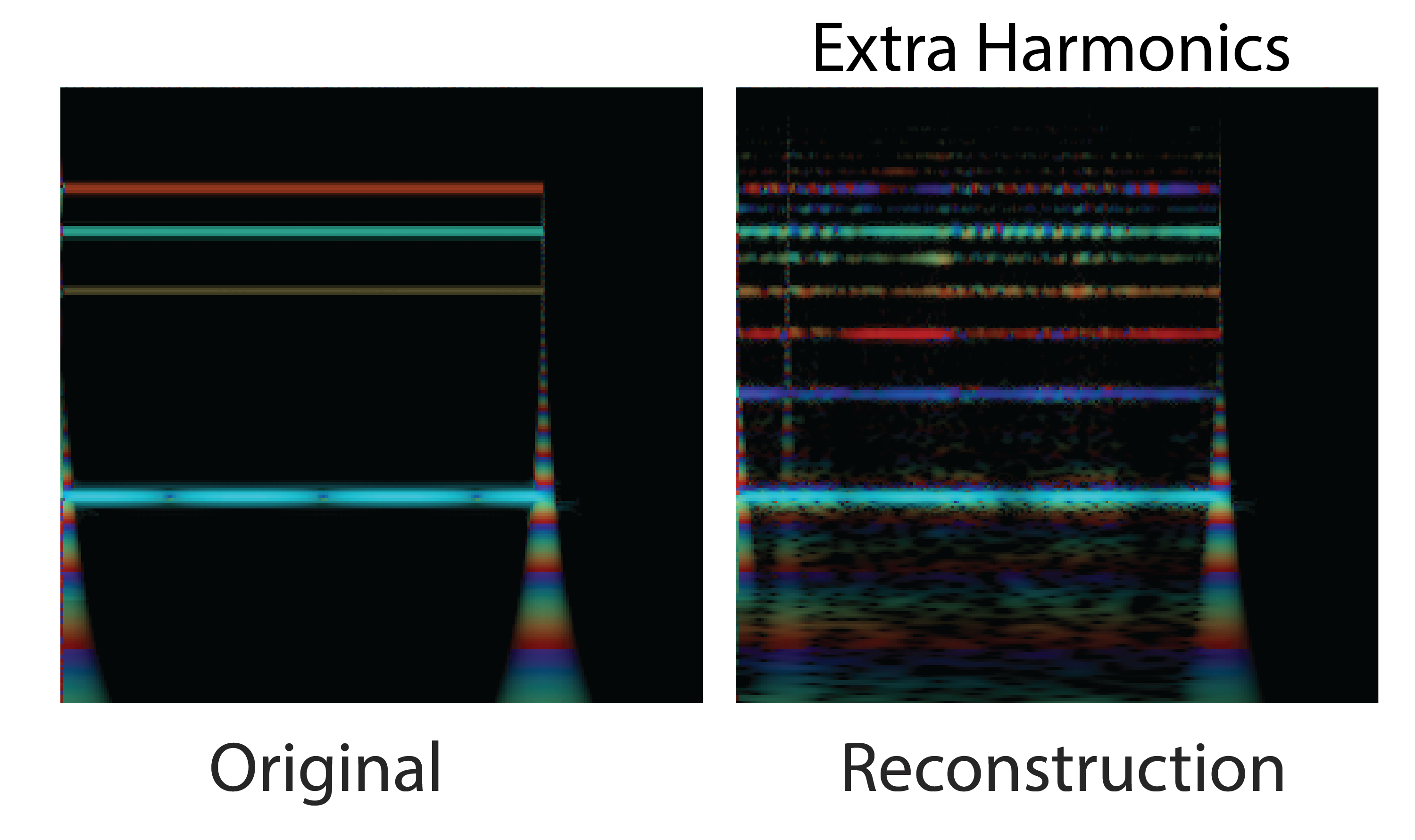
Since the algorithm is predicting one sample at a time, it is in essence drawing the waveform, and the mistakes it makes in its drawing result in upper harmonics that aren’t present in the original signal. While these harmonics aren’t “correct”, they are naturally plausible and have a very rich sound. Guitar distortion was discovered by guitarists turning up their amps to saturation in search of similarly exaggerated harmonics. Many audiophiles still swear by tube amplification for this “warmth” and harmonic complexity that is added to the sound. It’s interesting to note that despite the fact that our system is entirely digital, it learns dynamics where this rich coloring of the sound is the natural failure mode. Ocassionally, the model will also “click” as it samples an extreme value with a low probability and then quickly corrects itself.

Some reconstructed sounds also seem to fluctuate in fundamental frequency. Maintaining a consistent rate of repetition requires modeling extremely long time dependencies on the order of tens of thousands timesteps, which the model does not do perfectly. When the frequency varies, it wobbles smoothly, as sudden large shifts in frequency are unlikely.

All these factors come together to give these neural synthesizers a unique and consistent sound and feel. Regardless of whether they’re moving between strings, winds, or synthesizers, there is a distinct character to the sound and morphing that is specific to this particular model and training procedure.

Exploring a Latent Representation of Sound

Similar to how a good instrument controls a large range of sound with a small number of intuitive parameters, compressed representations are meaningful if they produce a large range and are manipulable. We encourage our network to find such a representation (what we’ve been calling z) by forcing the sound through a bottleneck, so that the original 16kHz audio is transformed into a series of 16-dimensional vectors at ~30Hz (32ms per frame). Below are examples of some of these latent representations of sound.

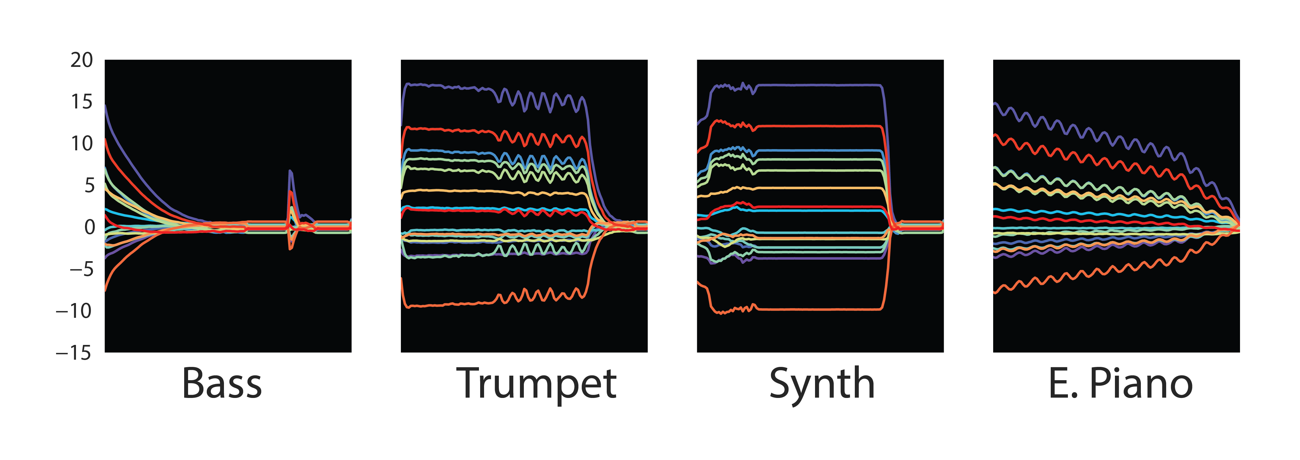
It’s interesting to note that the embeddings follow a similar dynamic envelope of the original sounds. Even some expressive information like vibrato is visible in the Trumpet figure above as quick fluctuations. Since we literally add this latent code to the layers of the WaveNet decoder network at generation time, it works like an excitation/activation of a nonlinear feedback system, and the network learns to be silent unless it receives this excitation. Viewed from a different perspective, the WaveNet is actually a very nonlinear infinite impulse response (IIR) filter that is being driven by the embeddings.

There’s a physical analogy that can be helpful in thinking about the system. Imagine standing in a fun-house version of an echo chamber. Your thoughts are the encoder, your voice is the embedding, and the resonance of the room is the WaveNet decoder. Everything is initially silent. You imagine a sound you want to make, interpret it with your voice, and start singing. As you sing, the room dynamically reshapes itself to mold the sound of the resonance into the sound you were thinking of initially.

As the embeddings seem to be driving the decoder, like the resonating room, we can explore what happens when we “turn up the volume” of the embeddings by just multiplying them with a linear coefficient. Below a threshold, the decoder spits and sputters but can’t form a consistent sound. As we multiply by numbers greater than one, the original sound becomes louder with more harmonic distortion, not unlike a guitarist overdriving a tube amplifier. Above a threshold, the whole system overloads and spends most the time clicking between extrema.

\[\begin{align} z_{new} = scaling * z \end{align}\]

The embeddings are a time-dependent signal, so we can shift our interpolations in time and listen to the resulting sounds. Below is the result of oscillating between two embeddings. The sound changes dynamically in a way that is clearly distinct from oscillating between the audio of the original sounds. Such expressive control could be enabled by real-time neural synthesis algorithms.

We can also try examining how sounds vary with their embeddings. If we look at the temporal mean and standard deviation across all the training notes, we see that the fine-scale structure of individual notes is smeared out. This manifests as a slow decay after both the initial attack and the release, as some notes in the dataset decay quickly and others take more time. The variance increases over time as well, reflecting this spread in decay times.

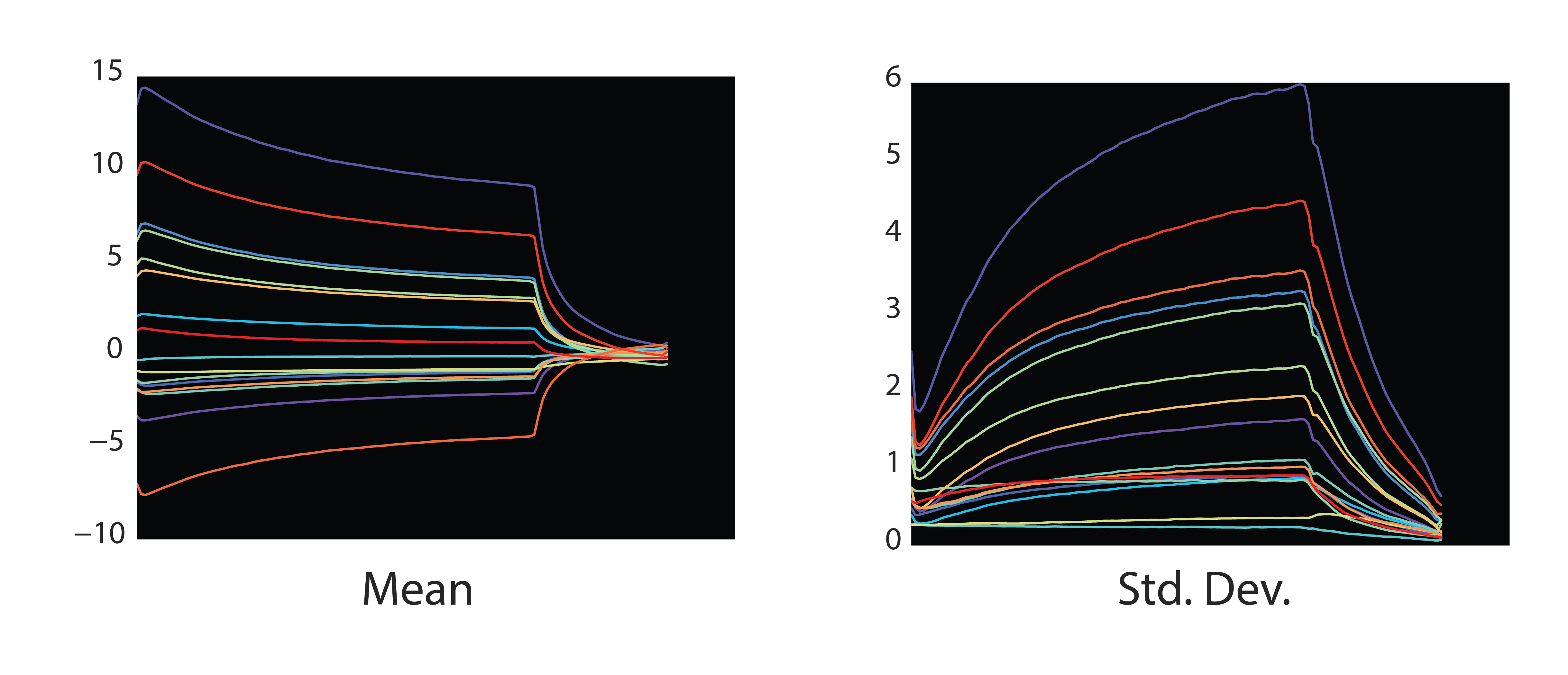
Interestingly, synthesizing this mean embedding sounds like a note from the dataset, but without much particular instrumental character. When the model fails to fit the particulars of an individual instrument, it ends up sounding like the mean.

Deviations from this mean give a sound its unique character. We can then create caricatures of sounds by linearly scaling the difference of an embedding from the mean embedding.

\[\begin{align} z_{new} = z_{mean} + scaling * (z - z_{mean}) \end{align}\]

We can also explore added noise to the embeddings and seeing how the sounds respond. Small amounts of noise create jitters and jolts out of equilibrium from which the model ocassionally recovers. Large amounts of noise dissolves the sound into tiny chunks and grains of audio.

\[\begin{align} z_{new} = z_{mean} + z_{std} * ( \frac{z - z_{mean}}{z_{std}} + \mathcal{N}(0, \sigma) ) \end{align}\]

While the model was trained on single instrument sounds, it can be applied to any sound of any length because it uses temporal embeddings that scale with the length of the sound. In the original post, we showed how we could reconstruct a sequence of notes even though the model was only trained on single notes. If we look at these reconstructions from a creative perspective, they create exciting and bizarre sounds when you apply NSynth way outside the realm it was trained on. The bias of the model and the data becomes an expressive filter to apply to any audio.

One example is reconstructing multiple notes played at a single time. The model has only seen a single harmonic series at a time, so it tries to capture polyphony by jumping between strong harmonics of an individual note.

Going further, what if we run a drum through NSynth? Having never seen percussive sounds, it does a surprisingly good job at reproducing acoustic and electronic drums. It only adds a small tonal bias. The exception is cymbals, which are so rich in harmonic structure that the model throws up its hands in entertaining ways.

These clips were created by reconstructing each drum sound independently and playing the virtual drum set with MIDI. Clips start with the original sounds and then follow with the reconstructed sounds.

Further still, what about the human voice? Electronic transformations of the voice have a long history (vocoders, autotune, etc.) and the model puts its own spin on this theme that is intelligible but also alien. Examples include Colin Raffel saying “Neural Synthesizer Instrument” and me saying “Hello world, I’m a synthesizer”.

These are just a couple toy examples of creative “misuses” of these technologies. The 808 only reached its full potential when artists repurposed it for themselves, and we can’t wait to see how people do the same for NSynth and other neural audio synthesis techniques.

Other Approaches

Finally, it’s worth mentioning that WaveNet autoencoders are just one particular model and interpolation is just one particular way of exploring latent spaces. In text and images, vector analogies are a powerful creative tool to manipulate specific aspects of media and explore spaces outside the training data. We tried generating sound from vector analogies of our embeddings. While the sounds were diverse, the temporal dimension of the embeddings led to less interpretable outcomes. Research is ongoing into hierarchical models that can chunk embeddings for a single sound into a single vector.

Autoregressive models like WaveNet are just one of many types of powerful generative models. The NSynth dataset was actually designed to mimic image datasets in size and focus so as to make it easier to transfer a range of image models to audio. For example, Generative Adversarial Networks (GANs) are quite popular for image processing but have yet to have significant success in modelling audio. They could be an ideal candidate to explore on the NSynth dataset.

Acknowledgements

Again, this work would not have been possible without fantastic collaborators in both the Google Brain team and DeepMind, especially Cinjon Resnick, Sander Dieleman, Karen Simonyan, and Adam Roberts. Thanks to Cinjon for help with editing and the sweet graphic of the instrument grid. Many thanks also to Yotam Mann, Teo Soares, and Alexander Chen at Google Creative Lab for bringing the Soundmaker to life. And finally, thanks to Colin Raffel for helpful ideas, beta testing many iterations of the instrument, and lending his voice to be robotified.