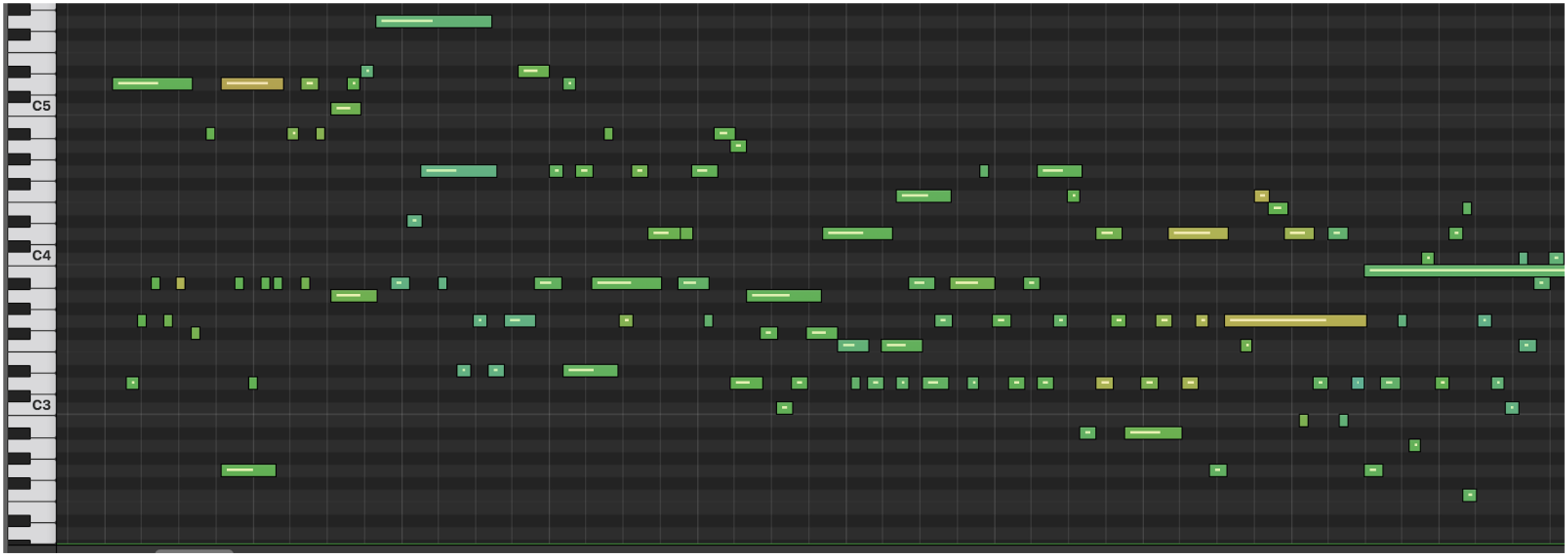
We present Performance RNN, an LSTM-based recurrent neural network designed to model polyphonic music with expressive timing and dynamics. Here’s an example generated by the model:

Note that this isn’t a performance of an existing piece; the model is also choosing the notes to play, “composing” a performance directly. The performances generated by the model lack the overall coherence that one might expect from a piano composition; in musical jargon, it might sound like the model is “noodling”— playing without a long-term structure. However, to our ears, the local characteristics of the performance (i.e. the phrasing within a one or two second time window) are quite expressive.

In the remainder of this post, we describe some of the ingredients that make the model work; we believe it is the training dataset and musical representation that are most interesting, rather than the neural network architecture.

Overview

Expressive timing and dynamics are an essential part of music. Listen to the following two clips of the same Chopin piece, the first of which has been stripped of these qualities:

The first clip is just a direct rendering of the score, but with all notes at the same volume and quantized to 16th notes. The second clip is a MIDI-recorded human performance with phrasing. Notice how the same notes lead to an entirely different musical experience. That difference motivates this work.

Performance RNN generates expressive timing and dynamics via a stream of MIDI events. At a basic level, MIDI consists of precisely-timed note-on and note-off events, each of which specifies the pitch of the note. Note-on events also include velocity, or how hard to strike the note.

These events are then imported into a standard synthesizer to create the “sound” of the piano. In other words, the model only determines which notes to play, when to play them, and how hard to strike each note. It doesn’t create the audio directly.

Dataset

The model is trained on the Yamaha e-Piano Competition dataset, which contains MIDI captures of ~1400 performances by skilled pianists. A prior blog post by Iman Malik also found this dataset useful for learning dynamics (velocities) conditioned on notes, while in our case we model entire musical sequences with notes and dynamics.

The Yamaha dataset possesses several characteristics which we believe make it effective in this context:

1. Note timings are based on human performance rather than a score.
2. Note velocities are based on human performance, i.e. with how much force did the performer strike each note?
3. All of the pieces were composed for and performed on one single instrument: piano.
4. All of the pieces were repertoire selections from a classical piano competition. This implies certain statistical constraints and coherence in the data set.

We have also trained on a less carefully dataset having the first three of the above characteristics, with some success. Thus far, however, samples generated by models trained on the Yamaha dataset have been superior.

Representation

Our performance representation is a MIDI-like stream of musical events. Specifically, we use the following set of events:

• 128 note-on events, one for each of the 128 MIDI pitches. These events start a new note.
• 128 note-off events, one for each of the 128 MIDI pitches. These events release a note.
• 100 time-shift events in increments of 10 ms up to 1 second. These events move forward in time to the next note event.
• 32 velocity events, corresponding to MIDI velocities quantized into 32 bins. These events change the velocity applied to subsequent notes.

The neural network operates on a one-hot encoding over these 388 different events. A typical 30-second clip might contain ~1200 such one-hot vectors.

It’s worth going into some more detail on the timing representation. Previous Magenta models used a fixed metrical grid where a) output was generated for every time step, and b) the step size was tied to a fixed meter e.g. a 16th note at a particular tempo. Here, we discard both of those conventions: a time “step” is now a fixed absolute size (10 ms), and the model can skip forward in time to the next note event. This fine quantization is able to capture more expressiveness in note timings. And the sequence representation uses many more events in sections with high note density, which matches our intuition.

One way to think about this performance representation is as a compressed version of a fixed step size representation, where we skip over all steps that consist of “just hold whatever notes you were already playing and don’t play any new ones”. As observed by Bob Sturm, this frees the model from having to learn to repeat those steps the desired number of times.

Preprocessing

To create additional training examples, we apply time-stretching (making each performance up to 5% faster or slower) and transposition (raising or lowering the pitch of each performance by up to a major third).

We also split each performance into 30-second segments to keep each example of manageable size. We find that the model is still capable of generating longer performances without falling over, though of course these performances have little-to-no long-term structure. Here’s a 5-minute performance:

More Examples

The performance at the top of the page is one of the better ones from Performance RNN, but almost all samples from the model tend to have interesting moments. Here are some additional performances generated by the model:

Temperature

Can we control the output of the model at all? Generally, this is an open research question; however, one typical knob available in such models is a parameter referred to as temperature that affects the randomness of the samples. A temperature of 1.0 uses the model’s predicted event distribution as is. This is the setting used for all previous examples in this post.

Decreasing temperature reduces the randomness of the event distribution, which can make performances sound repetitive. For small decreases this may be an improvement, as some repetition is natural in music. At 0.8, however, the performance seems to overly fixate on a few patterns:

Increasing the temperature increases the randomness of the event distribution:

Here’s what happens if we increase the temperature even further:

Try It Out!

We have released the code for Performance RNN in our open-source Magenta repository, along with two pretrained models: one with dynamics, and one without. Magenta installation instructions are here.

Let us know what you think in our discussion group, especially if you create any interesting samples of your own.

An arXiv paper with more details is forthcoming. In the meantime, if you’d like to cite this work, please cite this blog post as

Ian Simon and Sageev Oore. "Performance RNN: Generating Music with Expressive
Timing and Dynamics." Magenta Blog, 2017.
https://magenta.tensorflow.org/performance-rnn

to differentiate it from the other music generation models released by Magenta. You can also use the following BibTeX entry:

@misc{performance-rnn-2017,
    author = {Ian Simon and Sageev Oore},
    title = {
        Performance RNN: Generating Music with Expressive Timing and Dynamics
    },
    journal = {Magenta Blog},
    type = {Blog},
    year = {2017},
    howpublished = {\url{https://magenta.tensorflow.org/performance-rnn}}
}

Acknowledgements

We thank Sander Dieleman for discussion and pointing us to the Yamaha dataset, and Kory Mathewson, David Ha, and Doug Eck for many helpful suggestions when writing this post. We thank Adam Roberts for discussion and much technical assistance.