Editorial Note: One of the most rewarding experiences when putting out something for the world to use is to see someone build upon it. This is why we were very excited to see that a year after we open-sourced the code and model checkpoints for an arbitrary image stylization network architecture, Reiichiro Nakano had ported the model to TensorFlow.js. We reached out to Rei after noticing his demo online and he graciously accepted to contribute his code and model checkpoint to Magenta.js as the seed of our new image library @magenta/image. In this post, he shares his experience porting a deep learning model to TensorFlow.js, as well as optimizing it for a fast browser experience.
Shortly after deeplearn.js was released in 2017, I used it to port one of my favorite deep learning algorithms, neural style transfer, to the browser. One year later, deeplearn.js has evolved into TensorFlow.js, libraries for easy browser-based style transfer have been released, and my original demo no longer builds. So I started looking for a new project.
One of the main points of feedback I received from the community was that people wanted to provide their own style images to be used for stylization. Most style transfer models in the browser, including mine, are based on Johnson, et al 2016, which requires training a separate neural network for each style image. This means that in order to create pastiches of their own artwork, artists would have to train a separate model and port it to the browser–a process that requires a powerful GPU, several hours of training, and non-trivial technical know-how. A more desirable solution would be to consider a model that can already perform fast style transfer on any pair of content and style, and port that to the browser.
The Model
After searching related literature for a while, I stumbled upon a paper by Ghiasi, et. al. called Exploring the structure of a real-time, arbitrary neural artistic stylization network. This paper extends Dumoulin, et. al.’s work, A Learned Representation For Artistic Style, which was described in both a Magenta blogpost and a Google Research blogpost.
Here is a short comparison between the two papers:
- Both utilize a style transfer network that can map from content image to stylized image. The specific style is chosen by providing the transfer network with a style-specific set of layer normalization parameters.
- In Dumoulin, et. al.’s work, these style-specific parameters are learned directly from a finite number of styles (32 in the original paper), while in Ghiasi, et. al., they are generated for any arbitrary painting via a separate neural network called the style prediction network.
- The style-specific parameters can be taken as a latent space of style, and we can “combine” different styles by taking the weighted average between style representations of multiple styles.
- Ghiasi et. al. allows interpolation between the style representation of arbitrary styles, and so lets us do something like control the stylization strength. This is done by calculating the style representation of both the content image and the style image, and taking their weighted average.
If you want to know more details about the algorithm, I highly recommend reading the above-mentioned papers and blog posts.
Porting the Model to TensorFlow.js
One of the reasons I chose to port this particular model for arbitrary style transfer was the existence of both an open source TensorFlow implementation and pre-trained models at the Magenta repository. This made it very easy to directly port the pre-trained networks to TensorFlow.js using TensorFlow.js converter.
The ported TensorFlow.js model exists as two separate networks: a style prediction network that generates the style representation from a style image and a style transfer network that takes the style representation and the content image as inputs to generate the stylized image. This configuration gives us direct access to the style representation and, as mentioned above, lets us do things like control the stylization strength and combine multiple styles.
Saving them as separate models also allows us to swap out either the style prediction network or the style transfer network with a more efficient implementation, as we will see in the next sections.
The ported style transfer network’s weights have a size of 7.9MB, while the ported style prediction network’s (based on Inception-v3) weights have a size of 36.3MB.
Distilling the Style Prediction Network
Despite their huge size, the ported networks are able to perform stylization in a few seconds on a modern laptop. Still, forcing users to download a total of 44.2MB every time they visit a site does not make for a very good web experience. This is where a technique called distillation comes in useful.
Distillation, introduced in Hinton et al, 2015, is an elegant technique to compress the knowledge learned by a large neural network into a smaller neural network. This is useful when we want to take a large trained model and deploy it in a resource-constrained environment, such as the browser. The distillation process itself is extremely simple: train the smaller neural network to directly replicate the outputs of the large network.
In our case, we want to compress the knowledge learned by the 36.3MB Inception-v3 based style prediction network into a smaller network. I opted to use MobileNetV2 as the distilled style prediction network. There are several reasons for this choice:
- In the original paper for MobileNet, the authors show good results for distillation.
- MobileNetV2 has a high-quality open-source implementation in the TensorFlow GitHub organization. This makes it easy to plug in to the original arbitrary style transfer code.
- MobileNetV2 models have been ported to TensorFlow.js and are proven to be quite fast, even on mobile devices.
After replacing the last layer of the MobileNetV2 model to output a tensor with the same dimensions as the style representation, we proceed to train the network in the following manner:
- Using a combination of Painter by Numbers and the Describable Textures Dataset as our data source, we sample a batch of style images as training inputs.
- The style images are run through both the Inception-v3 and MobileNetV2 style prediction networks to produce two style representations for each style image.
- The mean squared error of the two style representations is taken and used as the loss value for updating the weights of the MobileNetV2 network using Adam.
Shown below is a diagram of the training process:
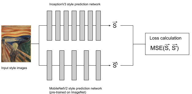
I stopped the training after around 73K parameter updates (compared to the 4M steps used to train the original models in the paper) as it was already showing satisfactory results. Note that I did not do any hyperparameter optimization for this distillation process, sticking with the defaults in the original code. It is entirely plausible that the distilled model can be further improved by simply running more parameter updates and/or doing some hyperparameter optimization.
After porting the distilled MobileNetV2 to TensorFlow.js, we end up with a style prediction network size of 9.6MB. Compared to the original 36.3MB, this is a size reduction of around 3.8x. This smaller model also naturally results in a speed improvement when predicting the style representation for an image:
| Checkpoint Size (MB) | Evaluation Time (s) | |
|---|---|---|
| Inception-v3 | 36.3 | 0.439 |
| MobilenetV2 | 9.6 | 0.047 |
While the evaluation times will vary by image size and system specs, my benchmark shows a nearly 9.3X improvement.
My code for doing this distillation is now available in the Magenta repo.
Shrinking the Style Transfer Network with Depthwise Separable Convolutions
After successfully reducing the model size of the style prediction network, I turned my attention to the style transfer network.
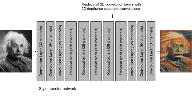
Despite the style transfer network’s weights taking up only 7.9MB of space, I was surprised to see that it was responsible for the majority (>95% for a 256x256x3 image) of the image stylization time. Looking closer at the architecture of the transfer network, we can see that it is mostly composed of 2D convolutional layers: 3 downsampling layers, 5 residual blocks of 2 convolutional layers each, and 3 upsampling layers. This is a total of 16 convolutional layers, with the middle 10 layers having 128 channels each.
One technique multiple papers have used to improve the efficiency of neural networks is to replace plain convolutional layers with depthwise separable convolutions. Developed by Laurent Sifre, there is a good reference to the history of depthwise separable convolutions in Section 2 of Chollet, 2016. Depthwise separable convolutions have been used as efficient “drop-in” replacements for convolutional layers, since they have fewer parameters and require less operations to compute.
I decided to switch out 13 convolutional layers of the model with depthwise separable convolutions, keeping the first 3 downsampling plain convolutional layers, as shown below:
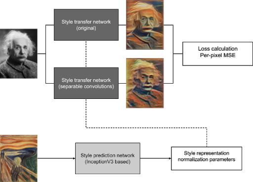
For training, I used distillation to train the depthwise separable convolution layers to reconstruct the per-pixel output of the original style transfer network, as shown in this diagram:
I stopped the training after around 110K updates when I thought the results looked acceptable, but again, it is likely that the model could be improved by training for a longer time and/or doing some hyperparameter optimization.
After porting the new style transfer network to TensorFlow.js, the total model size was only 2.4MB, a 3.3x reduction from 7.9MB. The evaluation time also improved by about ~2.8x.
| Checkpoint Size (MB) | Evaluation Time (s) | |
|---|---|---|
| Standards Convs | 7.9 | 2.51 |
| Depthwise Separable Convs | 2.4 | 0.90 |
Conclusion and Future Work
One reason I am open sourcing my code for distillation is so other interested people (with more resources) can take a shot at improving the distilled models. Since I don’t personally own a GPU for computation, I rely entirely on Google Colaboratory’s free GPU for training. Because of my limited resources, I have to be very selective of the ideas I actually implement. For those interested, however, here are a few ideas to improve these models:
- The original paper for distillation suggests adding a small term to the loss function, representing the real loss of the actual problem we are optimizing for. The intuition for this is as follows: since the smaller model cannot perfectly recreate the outputs of the bigger model, it helps to err in a direction minimizing the real loss of the actual problem. In our case, this real loss is the original style transfer loss derived from the VGG layer activations.
- Quantization is an easy way to reduce the size of the model weights. Instead of using the usual 32 bits to store the model weights, we can use 16 or even just 8 bits to reduce the model size. The TensorFlow.js converter makes this very easy by allowing us to set a quantization_bytes flag during conversion.
- In the style transfer network, I arbitrarily chose to replace the last 13 convolution layers with depthwise separable convolution layers. The speed of the model could be improved by switching the remaining layers to depthwise separable convolutions. On the the other hand, the quality may improve if we bring back some of the original convolution layers. I can imagine training multiple versions of this model and switching them out depending on the desired tradeoff between speed and quality.
- There exist other methods for arbitrary style transfer (e.g., 1 2 3 4 5). It would be interesting to see if the same techniques could be applied to bring these to the browser.
As a last note, I’d like to point out that I did not do anything particularly technically difficult to achieve these results. Distillation is fairly simple to implement yet I see few people using it to port models to the browser. My main hope is that this blog post inspires others to find similar low-hanging fruit and use these techniques to bring in more models from the wild into the browser.
About Me
I’m a software engineer working at a startup in Tokyo. Although my day job doesn’t involve machine learning, I enjoy the field and try to learn as much as I can about it during my limited free time. My main interests are machine learning for creativity and machine learning in the browser. Feel free to contact me if you want to collaborate on anything!
Postscript by Vincent Dumoulin
One appealing aspect of running a trained model in the browser is the breadth of devices that can be targeted: in an ideal world, any device equipped with a web browser would be able to run the model. In practice, hardware differences may complicate things a little: for instance, available memory may vary considerably between devices, which may make the model infeasible to run on lower-end devices.
In the course of publishing Rei’s exported model, we were reminded that not all devices support float32 computation: we noticed that the model would produce blank outputs on mobile phones whose GPUs only support float16 computation. Luckily for us, the underflow issues this caused were solvable by scaling up the value of certain weights in the model, however in general float16 underflow and overflow problems in models trained with float32 precision are not guaranteed to have such a simple solution.
If a model is likely to run on mobile devices, the best way to future-proof it is to keep this fact in mind when training and either train in float16 precision or regularize the model and set checks in place to ensure it can safely operate in float16 precision.